apparent motion also at 7T

WUSTL (ahem, WashU) recently set up a 7T scanner (Siemens Terra; 8Tx32Rx_Head_C head coil), and we've started a bit of piloting and exploring what we can do with it. I've been working through multiple aspects: the BOLD images themselves look different because of the stronger magnet, we're trying some new-to-me multi-echo sequences, collecting some noRF and phase images, and even the BIDS and fMRIPrep parts have taken some script updating. I think I'm getting enough of a handle on things now (thanks for help via neurostars, Chris Markiewicz and Taylor Salo!) to share some impressions, but it's all still very much in process.

We've had two pilot sessions so far, each with a different participant and somewhat different sequences. We're most interested in task fMRI, but that's tricky at the moment since the scanner doesn't (yet) have a way to present stimuli, nor to record responses. Eventually I want to do sequence comparisons with the reward-possible DMCC proactive Cued Task-Switching paradigm (and probably other tasks), like in my OHBM 2023 poster. But to get started I asked the second pilot participant to do a self-paced version of the HCP Motor task: blocks of right finger tapping, left finger tapping, right toe wiggling, left toe wiggling, tongue moving, with a bit of rest in between and a few deep breaths before and after each movement block to serve as onset/offset markers. (I'm not going to discuss the movement analysis parts yet, but so far I'm encouraged.)

Both pilot sessions included a pair (PA/AP) of runs with an acquisition similar-ish to what we used in the DMCC at 3T: 2.4 mm iso voxels, MB4, TR 1.2 s. But the 7T allows more acceleration, so they added in-plane acceleration (GRAPPA 2) and collected 4 echoes instead of just 1.

Below are the realignment parameters (from the fmriprep derivative _desc-confounds_timeseries.tsv files) for those runs from the two participants we've had so far. In both cases the grey vertical lines are at one-minute intervals; the first participant (TB7T1)'s runs were about 10.5 minutes and he alternated periods of regular and slow/deep breaths; the second participant (TD7T1)'s runs were about 6.5 minutes each and he did the blocked breathing-motor task.

TB7T1 clearly has much more apparent motion than TD7T1; the periods of regular and deep breathing are obvious, not only in the realignment parameters but also in movies of the BOLD run. TB7T1_run-44_echo-1_bold.avi is the "rawdata" (before preprocessing) version of echo 1; TB7T1_run-44_space-MNI152NLin2009cAsym_desc-preproc_bold.avi is after preprocessing (with fMRIPrep 25.1.0 using Tedana to optimally combine the echoes). The brain sort of looks like it's "jumping" with the breaths in the raw movie; perhaps more like expanding and contracting in the preprocessed version. 

The TB7T1 participant is the same individual as in some of our previous acquisition tests (at 3T); clearly, using 7T doesn't mean we can forget about apparent motion. ... I wouldn't have forgotten about apparent motion regardless since it's a favorite topic of mine, as is probably obvious since I'm starting off this (hopefully) series of posts about our 7T piloting with it.

Each of these sessions included multiple different acquisition sequences; in all cases TB7T1 had more obvious apparent motion than did TD7T1. TB7T1 run 28 had the largest apparent motion; it also had smaller voxels and a longer TR than the other examples.

Finally, the TB7T1 run 44 motion is also striking in the greyplot version created by fmriprep (left); TD7T1 run 24 is below, right:

reasonable motion censoring thresholds?

Recent participants have gotten me thinking (yet again) about the different types of motion during fMRI; causes and consequences. And more immediately practical: which motion censoring thresholds might be reasonable for particular tasks and analyses. 

I've long used (and recommended) FD > 0.9 as a censoring threshold for our event-related task fMRI studies (not functional correlation or resting state-type analyses). 0.9 is more lenient than many use for task fMRI; e.g., Siegel 2014: advise 0.5 FD for adults (which we have), 0.9 for kids or clinical populations. (I need to update a previous post; I'd misread Siegel's recommendations.)

Consider the following motion plot of a run from a recent participant, using my usual conventions (grey lines at one-minute intervals, frames along the x-axis); see this QC demonstration paper, the DMCC55B dataset descriptor, etc. for more explanation (and code). The lower panel shows FD, with the red line at the FD 0.9 censoring threshold, and red x marking censored frames; the grey horizontal line is at FD 0.5. 

I interpret this as a run with  minimal overt head motion, but pronounced apparent motion (from breathing, strongest in trans_y, consistent with the AP encoding direction). Zero frames are censored at an FD > 0.9 threshold (red line); 130 are censored at FD > 0.5 (grey line). There are 562 frames in the run, so 130/562 = 0.23 of the frames censored at FD 0.5, and we would drop the run at our usual criterion of < 20% censored frames.

Contrast the above plot with the following (marked with a 2 in the upper left); the same task, scanner, etc., but a different participant:

I'd characterize plot 2 as having more pronounced overt than apparent motion; there are oscillations in the trans_y, but these are dwarfed by the head motions, e.g., in the middle of the first minute. Looking at the censoring, 13 frames (corresponding to the largest overt head motions) are marked for censoring with FD 0.9; 40 are marked with FD 0.5, corresponding to more of the overt head motions. 40/562 = 0.07, well under the 20% censoring dropping threshold.

musings

To my eye, the 0.5 FD threshold is pretty reasonable in the second case, since it censors more of the overt head motion irregularities, and only those spikes. But for the first plot the 0.5 FD threshold seems far too aggressive: censoring part of every few breaths, 23% of the total frames. What do you think?

I hope to do some proper analyses of the impact of different amounts of apparent vs. overt motion on statistical analyses, but it is not a trivial problem, particularly with task entrainment. (Synchronizing breathing to task timing.)

As a final bit of food for thought, here are the tSNR and sd images for each of the two runs, without censoring (all 562 frames), after preprocessing, and with the same color scaling. The first strikes me as higher quality, despite the greater (> 0.5 FD) censoring. I believe apparent motion could have less of an impact on image quality than overt because the head is not actually moving, and so not creating the attendant magnetic disruptions; the differences are clear to the eye when viewing these types of runs as movies, but it's not clear how those differences translate to statistical analyses.

DMCC55B supplemental as tutorial: basic fMRI QC: motion

This is the third post in a series describing the DMCC55B supplemental files. The first introduces the dataset, and the second the questionnaire data. Here I'll highlight the first in the set of basic fMRI QC files: looking at the realignment parameters (head motion). 

While we use an FD threshold for censoring during the GLMs, I think plots with the six separate parameters are more useful for QC. These plots make up the bulk of QC_motion.pdf; one for each functional run included in DMCC55B. Chunk code5 of QC_motion.rnw creates these plots directly from the _desc-confounds_regressors.tsv produced during fmriprep preprocessing (note: newer versions name this file _desc-confounds_timeseries.tsv, but the columns used here are unchanged), and is relatively straightforward to adapt to other datasets; the code chunks between startup and code5 produce group summary statistics and can be omitted.

Above is the top of page 5 of the compiled file, including the motion plot for the first run. This shows very little overt or apparent motion, just a slight wiggle around frame 400 (8 minutes; grey lines are 1 minute intervals), which suggests they shifted during the break between the second and third task blocks (green horizontal lines). This run would be given an "A" (top) grade in our qualitative assessment.

f1659oa has extremely low overt head motion across this run, but clear apparent motion (breathing), primarily in the dark blue trans_y line.

R note: These motion (and the other) plots are made with base R graphics in a knitr document. The "stacked" 6-parameter and FD plots are made by using three par() commands within each iteration of the loop (chunk code5): first the size and margins for the upper plot; second the size and margins of the lower plot, with new=TRUE; finally, setting new=FALSE to finish and reset for the next run. 

yet more with respiration and motion regressors

Last year I did a series of posts on our experiences with multiband (SMS) task fMRI, particularly related to the respiration-related oscillations that are very apparent in the motion regressors of some people. See also practiCal fMRI's posts, especially this one. The tests and analyses here extend those, and convince me that the oscillations are not due to actual head motion, but rather B0 modulation or something else related to chest motion and/or blood oxygenation ("apparent head motion").

These scans are all using this previously-described MB4 acquisition sequence, and an experienced test person with rather prominent respiratory oscillations (the same person is in these first two plots) but little overt motion. We've been evaluating using Caseforge headcases to reduce movement and ensure consistent head positioning in the headcoil. We have two Caseforge headcases for this person: one fits quite tightly, and the other a little looser. This gives a set of comparison runs: with foam packing only (allowing more movement); with the regular Caseforge (some, but not much, movement possible); and with the tight Caseforge (motion essentially impossible).

The plots below show the 6 motion regressors (calculated from SPM12's realignment) and raw respiration signal (with a Siemens belt). I'm pretty confident that the motion regressors and respiration are precisely aligned here (it was approximate in some of last year's plots). The vertical grey lines mark one-minute intervals; the TR was 1.2 seconds. The tick marks show task onset; each run had three blocks of a verbal-response Stroop task.

First, here is a run without a headcase (normal packing). The difference in raw respiration amplitude between rest and task blocks is clear, as is some drifting over the course of the run. The y and z regressors closely match the respiration trace; hopefully you can zoom in to see that the y, z, and respiration curves are in phase - if the respiration curve goes up, both the y and z lines also go up. This was the case for all AP (anterior-posterior) encoded runs.

Next, here is a run of the same task and encoding (AP), with the very tight headcase. The oscillations in the y and z are still tightly matched to the respiration and about the same amplitude as before, but the drifting and rotation is quite reduced.

Finally, here is the same task, but the looser Caseforge headcase, and the reverse encoding (PA). The rotation is perhaps a bit more than with the tight headcase, but overall drift is quite low. The magnitude of the y and z oscillations is again about the same as the previous plots. If you look closely, the y line is out of phase from the respiration and z lines: the z line still goes up when the respiration goes up, but the y goes down.

We ran other tests, including some breath-holding. This is about two minutes of an AP and PA run breath-holding segment. The y-axis flipping is hopefully easier to see here: the blue peaks match the respiration peaks with AP, but fall in between on PA.

This y-axis flipping with encoding direction, plus the consistency of oscillation size across head stabilizers, has me convinced that we're seeing something other than overt head motion: I just don't believe he could have adjusted his y-axis movement with encoding direction that precisely, even had he known which encoding we were using each run.

If any of you have thoughts, or would like to look at these datasets to run additional tests, please let me know.

UPDATE 11 October 2018: This dataset is now available for download on openneuro.org, DOI:10.18112/openneuro.ds002737.v1.0.1 (was 10.18112/openneuro.ds001544.v1.1.0), called "multibandCFtests". (Note: I updated the links August 2020; the dataset was not properly deidentified the first time, requiring correction by the openneuro team - thanks!)

not all MB4 fMRI scans are free of gradients and banding

I was encouraged by the images in the previous post: it looked like the gradient and banding ("washing out") artifacts were not visible in the MB4 people. I need to revise that a bit: I do have bands and gradients in at least some MB4 people, though to a much lesser degree than in our MB8 datasets. How much this affects our task analyses is still to be determined.

On the left is the same MB4 person and run from the previous post (27 September 2017), voxelwise standard deviation over time of a task fMRI run, after going through the HCP minimal preprocessing pipelines. I was glad to see that the vessels were brightest (as they should be), though concerned about the frontal dropout. The person on the right is another person scanned at MB4 (doing the same task; same encoding, scanner, etc.); same preprocessing and color scaling for both.

The vessels clearly don't stand out as much in the person on the right. It's hard to tell in the above image, but there's a gradient in the standard deviation and tSNR images, with better signal on the edges than in the center of the brain. Below is another run from the person on the right, tSNR calculated on the images ready to go into afni for GLM calculation (so through the HCP minimal preprocessing pipelines, plus smoothing and voxelwise normalizing). This tSNR image is shown at six different color scalings; it's easier to see interactively (download the NIfTI here), but hopefully it's clear that the darker colors (lower tSNR) spreads from the center of the brain to the edges, rather than uniformly.

Here is the same person and run again, with the standard deviation (first two) and tSNR (right pane) of the raw (no preprocessing, first and lower) and minimally preprocessed (right two) images. I marked a banding distortion with green lines, as well as the frontal dropout. The banding is perfectly horizontal in the raw image, at 1/4 of the way up the image (see larger image), which makes sense, since this is an MB4 acquisition. I included the larger view of this raw image since all three banding artifacts are somewhat visible; in our dataset the inferior band is generally the most prominent.

The banding and gradient artifacts are certainly less visually prominent in our MB4 than our MB8 images, but they are present in some MB4 people. I haven't systematically evaluated (and probably won't be able to soon) all of our participants, so don't have a sense of how often this occurs, or how much it impacts detection of task BOLD (which is of course the key question).

Below the jump: movement regressors for the two runs in the top image; the person with the banding and gradients had very low motion; less than the person from the September post.

some thoughts on "Generation and Evaluation of a Cortical Area Parcellation from Resting-State Correlations"

Lately I've been working a bit with the brain parcellation map described in Gordon, et al. (2014), "Generation and Evaluation of a Cortical Area Parcellation from Resting-State Correlations" (citation below), which is available from the authors (thanks!) in both surface and volumetric formats.

As the title of the paper states, their brain parcellation was derived from resting state functional connectivity analyses. Briefly, the paper describes defining a set of ROIs ("parcels") which divide the cortical surface into meaningful (structurally and functionally) units. The parcel boundaries were defined from functional connectivity analyses, following the (reasonable) assumption that functional connectivity statistics should be homogenous within a parcel, but shift abruptly at parcel boundaries.

This is not the first functional connectivity-derived brain parcellation (Table 1 of the paper lists others), but I think is probably the most methodologically rigorous to date. I like that they used two datasets, each with more than 100 people, and serious quality control checks (motion, etc). I also like their reliability/stability/validity analyses: both between the two datasets, in individuals, and against the most robust and best understood atlases (including cytoarchitechtonic).

We'd like to use the parcellation for defining ROIs, particularly for frontal and parietal areas that aren't definitively divided in existing atlases. Gordon et al. did their analyses on the surface, but provide both surface (CIFTI) and volumetric (NIfTI) versions of the parcellation.

Here's an image I made (using a version of my knitr plotting code) showing a few slices the volumetric parcels (plotted on a conte MNI anatomy I resampled to 2x2x2 mm voxels to match the parcellation's resolution). As is apparent, while in volumetric space, the parcels closely follow the cortical surface (grey matter ribbon).

I see the logic of constraining analyses to the surface, particularly when fMRI images are acquired with high-resolution imaging and then subjected to precise, surface-optimized preprocessing (such as in the HCP). But I'm less convinced these narrow ROIs are advantageous for datasets collected with larger voxels (say 3x3x3 mm or larger) and "standard" preprocessing (such as SPM and spatial normalization).

For example, here are a few slices showing some of the validated ROIs from my recent paper overlayed on a few greyscale slices from the Gordon et al. parcellation. My dataset was acquired with 4x4x4 mm voxels, and all preprocessing was volumetric. The red ROI in the image at left was defined using a volumetric searchlight analysis, and, unsurprisingly, is rather "blobby:" it's not constrained to the cortical ribbon. The red ROI contains 416 voxels, of which 181 (.43) are in one of the parcels. Does that mean the 235 non-parcel voxels are uninformative? No. With 4x4x4 mm voxels, typical amounts of movement, and preprocessing which included spatial normalization, some of the BOLD, even if it all actually came from the grey matter, will appear to come from outside the cortical ribbon.

To summarize, my take is that this parcellation is the result of a methodological tour de force and worth careful consideration, especially for a high-resolution dataset preprocessed with surface analysis in mind (e.g. with freesurfer), even if doing a volumetric analysis. It may be less suitable for datasets with larger voxels and more standard preprocessing.


Gordon EM, Laumann TO, Adeyemo B, Huckins JF, Kelley WM, & Petersen SE (2014). Generation and Evaluation of a Cortical Area Parcellation from Resting-State Correlations. Cerebral cortex. PMID: 25316338 doi:10.1093/cercor/bhu239

hyperacuity with MVPA: a verdict yet?

A few years ago a debate started about whether MVPA hyperacuity is possible: can we pick up signals from sources smaller than an individual voxel? This topic popped up for me again recently, so this post organizes my notes, gives some impressions, and points out some of the key papers.

beginnings: V1 and grating orientations

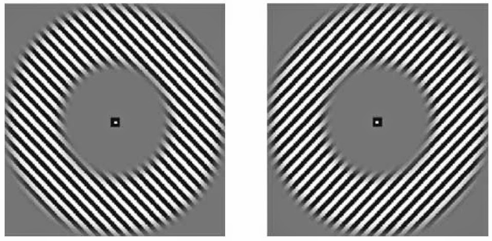
In 2005 Kamitani & Tong and Haynes & Rees reported being able to use MVPA methods with fMRI data to detect the orientation of gratings in V1. The anatomy and function of early visual areas is better understood than most parts of the brain; we know that they are organized into columns, each sensitive to particular visual attributes. In V1, the orientation columns are known to be much smaller than (typical) fMRI voxels, so how could classification be possible?

Multiple groups, including Kamitani & Tong in their 2005 paper, suggest that this "hyperacuity" could be due to a voxel-level bias in the underlying architecture, whether in the distribution of orientation columns, the vasculature, or some combination of the two. The idea here is that, since columns are not perfectly evenly spatially distributed, each voxel will end up with more columns of one orientation than another, and this subtle population-level bias  is what's being detected in the MVPA.

does degrading the signal reduce hyperacuity?

From the beginning, the idea that hyperacuity was behind the detection of orientation was met with both excitement and skepticism. In 2010 Hans op de Beeck wrote a NeuroImage Comments and Controversy article which kicked off a series of papers trying to confirm (or not) hyperacuity by means of degrading the fMRI images. The logic is straightforward: if subtle biases within individual voxels are making the classification possible, degrading the images (blurring, adding noise, filtering), should dramatically reduce the classification accuracy.

op de Beeck (2010) smoothed images with information at varying spatial scales at different FWHM to change their signal, interpreting the results as suggesting that the apparent hyperacuity might actually be due to larger-scale patterns (spanning multiple voxels). Objections to this technique were raised, however, partly because smoothing's affect on information content is complex and difficult to interpret. Swisher et al. (2010) used spatial filters, rather than smoothing, to degrade the signal in very high-resolution images, and found that small (< 1 mm) scale information was present, and critical for classification accuracy. But, the presence of small-scale signal in high-resolution images doesn't preclude the presence of larger (> 2 mm) scale information; indeed, larger-scale information was also found by Swisher et al. (2010). Filtering was also used by Freeman et al. (2011), who identified larger ("coarser") scale information about orientation in V1. Alink et al. (2013) also used filtering, along with more complex stimuli, finding information in a range of scales, but also cautioning that the numerous interactions and complications mean that filtering is not a perfect approach.

spiraling around

Recently, a set of studies have tried another approach: changing the stimuli (such as to spirals) to try to avoid potential confounds related to the visual properties of the stimuli. These debates (e.g., Freeman et al. 2013, Carlson 2014)  get too much into details of visual processing for me to summarize here, but a new set of Comments and Controversy NeuroImage articles (Carlson & Wardle, Clifford & Mannion 2015) suggests that using spiral stimuli won't be definitive, either.

my musings, and does this imply anything about MVPA?

Overall, I'm landing in the "bigger patterns, not hyperacuity" camp. I find the demonstrations of larger-scale patterns convincing, and a more plausible explanation of the signal, at least for human fMRI with ~ 3 mm voxels; it strikes me as equally reasonable that very small-scale patterns could dominate for high-resolution scanning in anesthetized animals (e.g., Swisher et al. 2010).

But do these debates imply anything for the usefulness of MVPA as a whole? Carlson and Wardle (2015) suggest that it does, pointing out that at this 10-year anniversary of the first papers suggesting the possibility of hyperacuity, we still haven't "determined the underlying source of information, despite our strong understanding of the physiology of early visual cortex." I wonder if this is because the best understanding of the physiology of early visual cortex is at the fine scale (neurons and columns), not the coarse scale ( > 5 mm maps). I agree that interpreting the properties of individual voxels from MVPA is fraught with difficulty; interpreting the properties of groups of voxels is much more robust.

papers mentioned here, plus some other relevant papers

• Alink, A., Krugliak, A.,Walther, A., and Kriegeskorte, N. (2013). "fMRI orientation decoding in V1 does not require global maps or globally coherent orientation stimuli." Frontiers in Psychology. doi:10.3389/fpsyg.2013.00493 
• Beckett, A., et al. (2012) "Contribution of large scale biases in decoding of direction-of-motion from high-resolution fMRI data in human early visual cortex." NeuroImage. doi:10.1016/j.neuroimage.2012.07.066
• Carlson, TA. (2014). "Orientation Decoding in Human Visual Cortex: New Insights from an Unbiased Perspective." J Neuroscience. doi:10.1523/JNEUROSCI.0548-14.2014
• Carlson, TA and Wardle, SG. (2015). "Sensible Decoding." NeuroImage. doi:10.1016/j.neuroimage.2015.02.009
• Clifford, CWG and Mannion, DJ. (2015). "Orientation decoding: Sense in spirals?" NeuroImage. doi:10.1016/j.neuroimage.2014.12.055
• Freeman, J et al. (2011). "Orientation Decoding Depends on Maps, Not Columns" J Neuroscience. doi:10.1523/JNEUROSCI.5160-10.2011
• Freeman, J. Heeger, DJ,Merriam, EP. (2013). "Coarse-Scale Biases for Spirals and Orientation in Human Visual Cortex." J Neuroscience. doi: 10.1523/JNEUROSCI.0889-13.2013
• Haynes, JD. and G. Rees (2005). "Predicting the orientation of invisible stimuli from activity in human primary visual cortex." Nat Neuroscience. doi:10.1038/nn1445
• Kamitani, Y. and F. Tong (2005). "Decoding the visual and subjective contents of the human brain." Nat Neuroscience. doi:10.1038/nn1444
• Kriegeskorte, N., R. Cusack, et al. (2010). "How does an fMRI voxel sample the neuronal activity pattern: Compact-kernel or complex spatiotemporal filter?" NeuroImage. doi:10.1016/j.neuroimage.2009.09.059
• Kubilius, J. and Baeck, A. (2010) "From What Scale of Representation Does Multivariate Pattern Analysis Decode Information?" J Neuroscience. doi:10.1523/JNEUROSCI.1153-10.2010
• Gardner, J. (2010). "Is cortical vasculature functionally organized?" NeuroImage. doi:10.1016/j.neuroimage.2009.07.004
• Op de Beeck, H. P. (2010). "Against hyperacuity in brain reading: Spatial smoothing does not hurt multivariate fMRI analyses?" NeuroImage. doi:10.1016/j.neuroimage.2009.02.047
• Op de Beeck, H. P. (2010). "Probing the mysterious underpinnings of multi-voxel fMRI analyses." NeuroImage. doi:10.1016/j.neuroimage.2009.12.072 
• Swisher, JD, et al. (2010). "Multiscale Pattern Analysis of Orientation-Selective Activity in the Primary Visual Cortex." J Neuroscience. doi:10.1523/JNEUROSCI.4811-09.2010