"Classification Based Hypothesis Testing in Neuroscience", permuting

My previous post described the below-chance classification part of a recent paper by Jamalabadi et. al; this post will get into the parts on statistical inference and permutation testing.

First, I fully agree with Jamalabadi et. al that MVPA classification accuracy (or CCR, "correct classification rate", as they call it) alone is not sufficient for estimating effect size or establishing significance. As they point out, higher accuracy is better, but it can only be directly compared within a dataset: the number of examples, classifier, cross-validation scheme, etc. all influence whether or not a particular accuracy is "good". Concretely, it is very shaky to interpret a study as "better" if it classified at 84% while a different dataset in a different study classified at 76%; if, however, you find that changing the scaling of a dataset improves classification (of a single dataset) from 76 to 84%, you'd be more justified in calling it an improvement.

The classification accuracy is not totally meaningless, but you need something to compare it to for statistical inference. As Jamalabadi et. al put it (and I've also long advocated), "We propose that MVPA results should be reported in terms of P values, which are estimated using randomization tests."{Aside: I think it's ok to use parametric tests for group-level inference in particular cases and after checking their assumptions, but prefer permutation tests and think they can provide stronger evidence.}

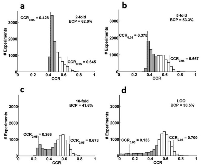
But there's one part of the paper I do not agree with, and that's their discussion of the prevalence of highly non-normal null distributions. The figure at left is Figure 5 from the paper, and are very skewed and non-normal null distributions resulting from classifying simulated datasets in different ways (chance should be 0.5). They show quite a few skewed null distributions from different datasets in the paper, and in the Discussion state that, "For classification with cross-validation in typical life-science data, i.e., small sample size data holding small effects, the distribution of classification rates is neither normal nor binomial."

However, I am accustomed to seeing approximately normal null distributions with MVPA, even in situations with very small effects and sample sizes. For example, below are null distributions (light blue) from eight simulated datasets. Each dataset was created to have 20 people, each with 4 runs of imaging data, each of which has 10 examples of each of 2 classes, and a single 50-voxel ROI. I generated the "voxel" values from a standard normal, with varying amounts of bias added to the examples of one class to allow classification. Classification was with leave-one-run-out cross-validation within each person, then averaging across the runs for the group-level accuracy; 1000 label rearrangements for the permutation test, following a dataset-wise scheme, averaging across subjects like in this demo.

The reddish line in each plot is the accuracy of the true-labeled dataset, which you can see increases from left to right across the simulated datasets, from 0.51 (barely above chance) to 0.83 (well above chance). The permutation test (perm. p) becomes more significant as the accuracy increases, since the true-labeled accuracy shifts to the right of the null distribution.

Note however, that the null distributions are nearly the same and approximately normal for all eight datasets. This is sensible: while the amount of signal in the simulated datasets increases, they all have the same number of examples, participants, classification algorithm (linear SVM, c=1), and cross-validation scheme. The different amounts of signal don't affect the permutation datasets: since the labels were randomized (within each subject and run), all permutation datasets are non-informative, and so produce similar null distributions. The null distributions above are for the group level (with the same dataset-wise permutation relabelings used within each person); I typically see more variability in individual null distributions, but with still approximate normality.

I suspect that the skewed null distributions obtained by Jamalabadi et. al are due either to the way in which the labels were permuted (particularly, that they might not have followed a dataset-wise scheme), or to the way the datasets were generated (which can have a big impact). Regardless, I have never seen as highly-skewed null distributions in real data as those reported by Jamalabadi et. al.



Jamalabadi H, Alizadeh S, Schönauer M, Leibold C, & Gais S (2016). Classification based hypothesis testing in neuroscience: Below-chance level classification rates and overlooked statistical properties of linear parametric classifiers. Human brain mapping, 37 (5), 1842-55 PMID: 27015748

demo: R code to perform a voxelwise t-test

It's easy to perform a voxelwise t-test (t-test at each voxel individually). Programs for mass-univariate analysis (like SPM and fsl) of course do this (and much more), but sometimes you just want to do a simple t-test across subjects at each voxel.

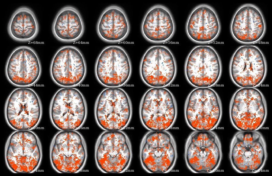
The demo code linked in this post does a voxelwise t-test in R. It takes as input a set of 3d NIfTI files, where each NIfTI is assumed to come from a different person, each voxel of which contains a statistic describing effect strength (for example, accuracy resulting from a searchlight analysis). The code reads the 3d NIfTI images into a 4d array (people in the fourth dimension), then performs a t-test at each voxel, saving the t-values for each voxel in a new NIfTI image. This figure shows the t-value image produced by the demo code.

UPDATE 4 June 2021:

The original version of this post continues below. I wrote a new version of the code to 1) avoid aaply (memory usage a bit better), and 2) use the RNifti instead of oro.nifti library (RNifti functions can be dramatically faster, and have some nice features; I now use RNifti exclusively for nifti image R input/output). I also added the files to the MVPA Meanderings OSF site, under the "voxelwise" subdirectory (direct link to R script).

Both versions of this code loop through all of the image voxels, which is most assuredly not the most efficient (or foolproof) way to perform a voxelwise t-test (I would recommend 3dttest++ instead, perhaps following 3dbucket; calling afni functions directly from R can make things quite smooth for those of us that are not bash fluent). I rewrote rather than removed this demo, however, because sometimes looping through all the voxels like this is the most straightforward way to get something done. 

permutation schemes: leave-one-subject-out

I've posted before about permutation schemes for the group level; here's an explicit illustration of the case of leave-one-subject-out cross-validation, using a version of these conventions. I'm using "leave-one-subject-out" as shorthand to refer to cross-validation in which partitioning is done on the participants, as illustrated here.

This diagram illustrates a fMRI dataset from two tasks and four participants, with one example of each task per person. Since there are four participants there are four cross-validation folds; here, the arrows indicate that for the first fold the classifier is trained on data from subjects 2, 3, and 4, while subject 1's data makes up the test set. The overall mean accuracy results from averaging the four accuracies (see this for more explanation).

How to get a significance value for the overall mean accuracy (grey oval)? We can't just do a t-test (or binomial) over the accuracies we got by leaving out each person (as often done after within-subjects classification), because the accuracies are not at all independent: we need a test for the final mean accuracy itself.

My strategy is to do dataset-wise permutation testing by label-flipping within one or more participants each fold. In this case, there are only four participants, so we could flip labels in just one or two of the participants, for 10 possible permutations (choose(4,1) + choose(4,2)) (flipping all the subjects' labels would recreate the original dataset, since this is dataset-wise permutation testing.) Here, the task labels for participant 1 only are flipped (the first example becomes task 2, the second, task 1). The entire cross-validation then proceeds with each flipped-labels dataset.

 I follow the same strategy when there are more than one example of each class per person: when the person's labels are to be 'flipped' for a permutation I relabel all the class 1 examples as class 2 (and class 2 as class 1). While the number of possible permutations is limited by number of participants in this scheme, it increases rapidly with the number of participants.

Anyone do anything different?

"jumping stars": a side effect of low power

In brief, statistical power refers to the long-run frequency of rejecting H0 and accepting H1 (if the experiment was repeated), when the truth is that the effect exists - the null hypothesis should be rejected. Unfortunately, psychological and neuroimaging studies tend to be underpowered. There are plenty of practical and historical reasons for this, see the references listed below for readable introductions.

In this post I'll demonstrate one side effect of low-powered studies: reproducing results can be very difficult, even when the effects actually exist. I sometimes refer to this effect as "jumping stars", for reasons that will become apparent. This example is adapted from one presented in Maxwell (2004).

example

Suppose that we want to test if depression level is related to “self-perceived competence” in academic, appearance, athletic, behavioral, and social domains. To answer this question, we measure the depression level and those five domains of self-perceived competence in 100 people.

Once we have the data, we do a multiple linear regression to see which competence areas are most related to the depression score. (The variables are scaled in such a way that positive regression coefficients imply that higher levels of perceived competence correspond to lower levels of depression.)

For concreteness, here's the data for the first few (pretend) people:

Now we do the linear regression, and get the following:

What can we conclude? Well, it looks like higher levels of athletic and social perceived competence are associated with lower levels of depression. These p-values are quite good, surviving even a Bonferroni correction for multiple comparisons.

Now, someone decides to replicate our study, and measures depression and self-perceived competence in 100 different people. They got this result from the linear regression:

And another study's results:

Oh no! Things are not replicating very well .... to summarize:

What happened? As you probably guessed from my introduction about power, these three studies are not "bad" or finding non-existent effects, but rather are underpowered.

These three datasets were created when I ran the same simulation (R code here) three times. The simulation creates an underpowered study in which the factors are equally important: all five measures are correlated at 0.3 with the depression score.

Thus, all factors should be found equally important. But we don’t have enough power to find them all, so we only find a few in each individual study. The results of each study are thus not exactly incorrect, but rather incomplete, and unstable: which effects were detected in each varied randomly.

And that is why I refer to this effect as "jumping stars": which row of the results table gets the stars (is found significant) varies as it is repeated; the significance stars seem to jump around unpredictably.

comments

There is no easy fix for the jumping stars problem, since it's due to the hard-to-solve problem of low statistical power. And it can be quite difficult to distinguish this situation - true effects but low power - from a situation in which replication fails because the effects are nonexistent (due to random chance).

As Maxwell (2004) explains (and you really should read it if you haven't), jumping stars cause much more problems when many analyses are performed, since, when the truth is that the effects are real, the likelihood that a low-powered study will find one of the effects significant is much, much larger than the likelihood that the study will find all of the effects significant (which is actually the truth).

All of this can add up to a messy, unstable, contradictory literature in which replication is very difficult - even if the effects actually are present!

But I am not counseling despair, rather awareness and caution. We must be very, very cautious in interpreting negative results; aware that many true effects could have been missed. And we should keep power in mind when designing experiments and analyses: more is generally better.

some references

Maxwell, S.E. (2004). The persistence of underpowered studies in psychological research: Causes, consequences, and remedies. Psychological Methods, 9, 147-163.

Sedlmeier & Gigerenzer, 1989. Do Studies of Statistical Power have an Effect on the Power of Studies?

Yarkoni, T. (2009). Big Correlations in Little Studies: Inflated Correlations Reflect Low Statistical Power. Perspectives on Psychological Science, 4, 294 - 298.

"ironic" comments on cross-validation

There is an interesting set of responses to "Ten ironic rules for non-statistical reviewers" (Friston, 2012) in press at NeuroImage. Many interesting issues are raised, but I want to touch on the discussion of cross-validation in the reply Sample size and the fallacies of classical inference (Friston, 2013).

from Friston, 2013:

"Is cross validation useful?
[...] I think that the role of cross validation in neuroimaging deserves further discussion. As articulated clearly by Lindquist et al., the goals of inference and cross validation are very distinct. Cross validation is generally used to validate a model (or its parameters) that predicts or classifies using new observations. Technically, this is usually cast in terms of a posterior predictive probability density. Cross validation is used to validate this posterior predictive density for diagnostic or other purposes (such as out-of-sample estimation or variable selection). However, these purposes do not include model comparison or hypothesis testing. In other words, cross validation is not designed for testing competing hypotheses or comparing different models. This would be no problem, were it not for the fact that cross validation is used to test hypotheses in brain mapping. For example, do the voxels in my hippocampal volume of interest encode the novelty of a particular stimulus? To answer this question one has to convert the cross validation scheme into a hypothesis testing scheme - generally by testing the point null hypothesis that the classification accuracy is at chance levels. It is this particular application that is suboptimal. The proof is straightforward: if a test of classification accuracy gives a different p-value from the standard log likelihood ratio test then it is – by the Neyman–Pearson Lemma – suboptimal. In short, a significant classification accuracy based upon cross validation is not an appropriate proxy for hypothesis testing. It is in this (restricted) sense that the Neyman–Pearson Lemma comes into play.

I have mixed feelings about cross validation, particularly in the setting of multivariate pattern classification procedures. On the one hand, these procedures speak to the important issue of multivariate characterisation of functional brain architectures. On the other hand, their application to hypothesis testing and model selection could be viewed as a non-rigorous and slightly lamentable development."

I fully agree that "cross validation is not designed for testing competing hypotheses or comparing different models", but do not see how that is a problem for (typical) MVPA hypothesis testing.

This image is my illustration of a common way cross-validation is used in MVPA to generate a classification accuracy (see this post for an explanation). As Friston says in the extract, we often want to test whether the classification accuracy is at chance. My preferred approach in these sorts of cases is usually dataset-wise permutation testing, in which the task labels are changed, then the classification (and averaging the accuracies obtained on the cross-validation folds) is repeated, resulting in a null distribution for mean accuracy to which the true mean accuracy can be compared (and a significance level obtained, if desired).

In this scenario the cross-validation does not play a direct role in the hypothesis testing: it is one step of the procedure that led from the data to the statistic we're hypothesizing about. The classification accuracy is not significant "based upon cross validation", but rather significant based on the permutation testing; cross-validation is one stage of the procedure that led to the classification accuracy.


Friston, K. (2013). Sample size and the fallacies of classical inference NeuroImage DOI: 10.1016/j.neuroimage.2013.02.057

MVPA Permutation Schemes: Permutation Testing in the Land of Cross-Validation

Next week I will be attending PRNI 2013, presenting "MVPA Permutation Schemes: Permutation Testing in the Land of Cross-Validation". The papers will be published, but are not online yet. I'll add a link once one's online, but let me know if you'd like a copy now and I'll send you a pdf. The little demo accompanying the paper is already online, here (it's a zip, containing a pdf explanation plus knitr R code and files). I'd like to expand the paper to include more examples and firmer advice, but the little paper is a (hopefully) a clear overview of the issues.

The paper describes a few ways in which permutation testing is commonly done in MVPA, focusing on how the cross-validation folds (aka data partitions) are accounted for. If you're not familiar with why cross-validation is relevant for MVPA, I think this is a pretty readable statistically-oriented introduction, you could try a paper I wrote a few years ago (Etzel, J.A., Gazzola, V., Keysers, C., 2009. An introduction to anatomical ROI-based fMRI classification analysis. Brain Research 1282, 114-125.), or just google.

two permutation schemes

One goal of the paper is to point out that "we did a permutation test" is not a sufficient description for MVPA, since there are many reasonable ways to set up permutation tests. We use the terms "dataset-wise" and "fold-wise" to describe two common schemes. Since these terms aren't standard, we illustrate the two schemes with a running example.

introduction: running example

The running example is based on what I think is pretty much the simplest situation possible for task-based classification analysis for a single subject:

"This person completed three runs of fMRI scanning, each of which contained three blocks each of two different tasks. These task blocks were presented with sufficient rest intervals to allow the task-related BOLD signal to return to baseline, making it reasonable to assume that the task labels can be permuted [2, 3]. We further assume that the image preprocessing (motion correction, etc.) was adequate to remove most linear trends and uninteresting signals. Temporal compression [4] was performed, so that each task block is represented in the final dataset as a single labeled vector of voxel values (Fig. 1). There are n entries in each vector, corresponding to the voxels falling within an anatomically-defined region of interest (ROI). We assume that n is small enough (e.g. 100) that further feature selection is not necessary.

We wish to use a classification algorithm (e.g. linear support vector machines) to distinguish the two tasks, using all n voxels listed in the dataset. For simplicity, we will partition the data on the runs (three-fold CV): leave out one run, train on the two remaining runs, and repeat, leaving out each run in turn. The three test set accuracies are then averaged to obtain the overall classification accuracy (Fig. 2), which, if greater than chance, we interpret as indicating that the voxels’ BOLD varied with task."

I carry this way of illustrating cross-validation and classification through the later figures. The white-on-black color indicates that these examples have the true task labels: the numbers in the circles (which are 'seen' by the classifier) match those of the third (task) column in the dataset.

permutation schemes

Now, the permutation testing. We need to put new task labels on, but where? There are 20 ways of reordering the task labels; shown in the figures as colored circles on a light-grey background.

Under the dataset-wise scheme we put the new task labels on before the cross-validation, carrying the new labels through the cross-validation folds. Figure 4 shows how this works when both the training and testing sets are relabeled, while Figure 5 shows how it works when only the training sets are relabeled.

Note that the dataset's structure is maintained under the dataset-wise permutation scheme when both training and testing sets are relabeled (Figure 4 has the same pattern of arrows as Figure 2). Some of the arrows are shared between Figure 5 and Figure 2, but the property (in the real data) that each labeling is used in a test set is lost.

Under the fold-wise permutation scheme we put the new task labels on during the cross-validation. Figure 6 shows this for relabeling the training data only, as suggested in the pyMVPA documentation. Figure 6 has a similar structure to Figure 5, but the coloring is different: under the dataset-wise scheme a run is given the same set of permuted labels in all training sets in a permutation, while under the fold-wise scheme each run gets a different set of permuted labels (i.e. in Figure 5 run 1 is purple in both the first and second cross-validation folds, while in Figure 6 run 1 is purple in the first and red in the second).

does the permutation scheme matter?

Yes, at least sometimes. We are often dealing with such small, messy datasets in MVPA that shifting the rank by just a few values can really matter. The simulations in the little demo show a few (tweakable) cases.

Here are the first two repetitions of the demo (this is in a more readable format in the pdf in the demo). In the first, the true-labeled accuracy was 0.64 (vertical line), the p-value for both.dset (permuting training and testing labels dataset-wise, ala figure 4) was 0.013, train.dset (dataset-wise, permuting training only, ala figure 5) was 0.002; both.fold (permuting both, fold-wise) was 0.001, and train.fold (fold-wise permuting training only, ala figure 6) was 0.005. On repetition 2, the p-values were: both.dset=0.061, train.dset=0.036, both.fold=0.032, and train.fold=0.028. That gives us p-values above and below the 'magical' value of 0.05, depending on how we do the permutation test.

final thoughts

Which permutation scheme should we use for MVPA? Well, I don't know a universally-applicable answer. As we know, how simulated datasets are created can really, really matter, and I certainly don't claim this little demo is representative of true fMRI data. That said, the pattern in null distributions above - larger variance on dataset-wise than fold-wise schemes (and so a more stringent test) - is common in my experience, and unsurprising. It seems clear that more of the dataset structure is kept under dataset-wise schemes, which is consistent with the goal of matching the permutation test as closely as possible to the true data analysis.

My feeling is that dataset-wise permutation schemes, particularly permuting both the training and testing sets (Fig. 4) is the most rigorous test for a dataset like the little running example here. Dataset-wise permuting of either just the training or just the testing set labels may be preferable in some cases, such as 'cross' classification, when the training and testing datasets are not runs but rather independent datasets (e.g. different experimental conditions or acquisition days).

I don't think that fold-wise schemes should be recommended for general use (datasets like the running example), since some of the dataset structure (similarity of training data across cross-validation folds) present in the true data is lost.

UPDATE (20 June 2013): Here is a link to a copy of my poster, plus expanded simulation code.

UPDATE (22 July 2013): Here is a link to a copy of the paper, as well.

UPDATE (6 November 2013): The paper is now up at IEEE and has the DOI 10.1109/PRNI.2013.44.

low-accuracy subjects' influence on group statistics

background

This post comes from something I saw in some of my actual searchlight results.The searchlight analysis was performed within a large anatomical area (~1500 voxels, svm within fairly small searchlights), separately in ~15 people. In most subjects, most all searchlights classified quite well, but in two subjects most searchlights classified quite poorly. As usual, there were a few low-accuracy searchlights in the "good" subjects (people in which most searchlights classified well), and a few high-accuracy searchlights in the "bad" subjects (people in which most searchlights did not classify accurately).

I made the group-level results by performing a t-test at each voxel: are the subjects' accuracies greater than chance? (I did not smooth the individual searchlight maps first.) I saw a worrisome pattern in the group maps: the peak (best t-value) areas tended to coincide where the "bad" subjects had their best (most accurate) searchlights. This outcome is not surprising (see below), but is not what we want: applying a strict threshold to the group map will identify voxels. But those particular voxels came out as peak because the "bad" subjects had accurate searchlights in those locations, not because the voxels were more accurate across subjects: the group map was overly influenced by the low-accuracy subjects.

simulation

Here's a little simulation to show the effect (R code is here). The code creates 15 searchlights, each of which contain 10 voxels. There are 12 people in the dataset, 10 of whom have signal in all searchlights, and 2 of whom have signal in all but the first two searchlights. It's a two-class classification, using a linear SVM, partitioning on the two "runs". Voxel values were sampled from a normal distribution, with different means for the voxels with signal but the same means for no signal.

The classification accuracies of the 12 people in each of the 15 searchlights are summarized in these boxplots (the figure should get larger if you click on it; run the code to get the underlying numbers). The accuracies vary a bit over the people and searchlights, as expected, given how the data was simulated. All of the "boxes" are well above chance, and all of the t-values (see figure labels) are above 5. So this seems reasonable.

The searchlights with the highest t-values are 1 and 2: the two searchlights which I assigned to have signal in the two "bad" subjects. You can see why in the boxplots: the bottom whisker in searchlights 1 and 2 only reach 0.6, while all the others have a whisker or outlier closer to chance. Some searchlights (like 8) have two outliers: the two "bad" subjects.

So the t-test didn't make an error: the first two searchlights should have the highest t-values, since they have the most individual accuracies the furthest above chance. But this could have led to an improper conclusion: If we had applied a high threshold (t > 8 in this simulation) we might think the first two searchlights are where the information falls, where in actuality it is evenly distributed.

what to do?

Follow-up testing or different group-level statistics can help to catch this type of situation. As often is the case, precise hypotheses are better (for example, if you want to find searchlights with significant classification in most subjects individually, test for that directly - don't assume that the best searchlights in a t-test will also have that property).

Here are a few suggestions for follow-up testing:

• Look at the individual subject's searchlight maps: Are a few subjects quite different than the rest (such as here, where two people had quite low accuracies compared to the others)? 
• Sensitivity testing can help: how much does the group-level map change when individual subjects are left out? 
• Do the group-level results align more closely with some subjects than others?

permutation testing: feedback

MS Al-Rawi sent some feedback about my last post and kindly agreed that I could post it here. His comments/questions are in quote blocks, my responses in regular type.

"1- The title: 'groups of people'. Are you trying to perform permutation testing for a group of subjects (people), so, is it 'groups of people', or group analysis?"

I meant group analysis (aka 2nd level analysis): "is this effect present in these subjects?" The goal is to generate a significance level for the group-level statistic, such as the accuracy averaged across subjects.

"2- You also wrote; 'Assume further that there is a single set of p unique relabelings (label permutations), applied such that there is a linking between the permutations in each person'. So, how do you get this set of  'p unique relabelings', or you don't have to find them, you just do find p times relabelings?"

Sorry for the confusion; I was struggling a bit with terminology. What I mean is that there is a single set of label permutations which are used for every person, rather than generating unique label permutations for everyone. The set of label permutations is created in the 'usual' way. If the number of labels is small all possible permutations should be used, but when there are too many for that to be practical a random subset can be generated.

For example, suppose there are two classes (a and b) and three examples of each class. If the true labeling (i.e. row order of the data table) is aaabbb, possible permutations include aabbba, ababab, etc.

"3- 'applied such that there is a linking between the permutations in each person'. I cannot figure out what that is? I can tell that it gives a biased distribution, either all yielding best accuracy(s) that are closer to the real one, or all yielding closer to chance level accuracy."

What I meant was that, if all subjects have the same number and type of examples, the same (single) permutation scheme can be used for everyone. To continue the example, we would calculate the accuracy with the aabbba relabeling in every subject, then the accuracy with the ababab relabeling, etc.

I guess this gives a biased distribution in the sense that fewer relabelings are included ... When a random subset of the permutations has to be used (because there are too many to calculate them all), under scheme 2 you could generate a separate set of permutations for each person (e.g. aabbba might be used with subject 3 but not subjects 1, 2, or 4). The single set of permutations used for everyone is not biased (assuming it was generated properly), but does sample a smaller number of relabelings than if you generate unique relabelings for each person.

"4- Since each person/subject (data) has its own classifier (or a correlated set of classifiers due to using k-fold cross validation), is it legitimate to take the mean of each of the 'p unique relabelings' (as you showed in scheme 1)?"

This is one of the reasons why I made the post: to ask for opinions on its legitimacy! It feels more fair to me to take the across-subjects mean when the same labeling is used for everyone than averaging values from different labelings. But a feeling isn't proof, and it's possible that scheme 1 is too stringent.

"5- The formula; ((number of permutation means) > (real mean)) / (r + 1)
I think using ((number of permutation means) > (real mean) +1 ) / (r + 1) would prevent getting p=0 value when the classification accuracy is highly above change. We shouldn't be getting 0 in any case, but that is most probably to happen because the number of permutations is limited by the computational power, and the randomization labeling might not be perfectly tailored enough to generate an idealistic distribution (e.g. at one permutation should capture the original labeling or one that is highly close to it and thus give high classification accuracy)."

Yes, I think this is right: if the true labeling is better than all 1000 permutations we want the resulting p-value to come out as 0.001, not 0.

permutation testing: groups of people

Here I describe three ways to do a group permutation test. The terminology and phrasing is my own invention; I'd love to hear other terms for these ideas.

First, the dataset.

I have data for n people. Assume there are no missings, the data is balanced (equal numbers of both cases), and that the number of examples of each case is the same in all people (e.g. 10 "a" and 10 "b" in each of three runs for every person).

For each person there is a single "real accuracy": the classification of their data with the true labeling. We can average these n values for the real group average accuracy.

Assume further that there is a single set of p unique relabelings (label permutations), applied such that there is a linking between the permutations in each person. In other words suppose relabeling 1 = abaabba ... aabbb. The "perm 1" box for each person is the accuracy obtained when relabeling 1 is used for that person's data; permutations of the same number for each person use the same relabeling.

Next, we generate the null distribution.

Here are the three schemes for doing a group permutation test. In the first, the linking between permutations described above is maintained: p group means are calculated, one for each of the p unique relabelings. I've used this scheme before.

Alternatively, we could disregard the linking between permutations for each person, selecting one accuracy from each person to go into each group mean. Now we are not restricted to p group means; we can generate as many as we wish (well, restricted by the number of subjects and permutations, but this is usually a very, very large number). In my little sketch I use the idea of a basket: for each of the r group means we pick one permutation accuracy from each person at random, then calculate the average. We sample with replacement: some permutations could be in multiple baskets, others in none. This is the scheme used in (part of) Stelzer, Chen, & Turner, 2012, for example.

Or, we could fill our baskets more randomly: ignoring the separation into subjects. In other words, we draw n permutation values each of r time, disregarding the subject identities. This is closer to the common idea of bootstrapping, but I don't know of any examples of using this with neuroimaging data.

Finally, the null distribution.

Once we have the collection of p or r group means we can generate the null distribution, and find the rank (and thus the p-value) of the real accuracy, as usual in permutation testing. To be complete, I usually calculate the p-value as ((number of permutation means) > (real mean)) / (r  + 1). I actually don't think this exact equation is universal; it's also possible to use greater-than-or-equal-to for the rank, or r for the denominator.

Thoughts.

I feel like the first scheme ("stripes") is the best, when it is possible. Feelings aren't proof. But it feels cleaner to use the same relabeling scheme in each person: when we don't, we are putting a source of variability into the null distribution (the label scheme used for each person) that isn't in the real data, and I always prefer to have the null distribution as similar to the real data as possible (in terms of structure and sources of variance).

A massive problem with the first scheme is that it is only possible when the data is very well-behaved: the same relabeling scheme can be applied to all subjects. As soon as even one person has some missing data, the entire scheme breaks. I've used the second scheme ("balanced baskets") in this case, usually by keeping the "striping" whenever possible, then bootstrapping the subjects with missing (This is sort of a hybrid of the first two schemes: I end up with p group means, but the striping isn't perfect).

A small change to the diagram gets us from the second to the third scheme (losing the subject identities). This of course steps the null distribution even further from the real data, but that is not necessarily a bad thing. Stelzer, Chen, & Turner (2012) describe their scheme 2 as a "fixed-effects analysis" (line 388 of the proof). Would scheme 3 be like a random-effects analysis?

So, which is best? Should the first scheme be preferred when it is possible? Or should we always use the second? Or something else? I'll post some actual examples (eventually).

permuting searchlight maps: Stelzer

Now to the proposals in Stelzer, not just their searchlight shape!

This is a dense methodological paper, laying out a way (and rationale) to carry out permutation tests for group-level classifier-based searchlight analysis (linear svm). This is certainly a needed topic; as pointed out in the article, the assumptions behind t-tests are certainly violated in searchlight analysis, and using the binomial is also problematic (they suggest that it is too lenient, which strikes me as plausible).

Here's my interpretation of what they propose:

1. Generate 100 permuted searchlight maps for each person. You could think of all the possible label (i.e. class, stimulus type, whatever you're classifying) rearrangements as forming a very large pool. Pick 100 different rearrangements for each person and do the searchlight analysis with this rearrangement. (The permuted searchlight analysis must be done exactly as the real one was - same cross-validation scheme, etc.)
2. Generate 100,000 averaged group searchlight maps. Each group map is made by picking one permuted map from each person (out of the 100 made for each person in step 1) and averaging the values voxel-wise. In other words, stratified sampling with replacement.
3. Do a permutation test at each voxel, calculating the accuracy corresponding to a p = 0.001 threshold. In other words, at each voxel you record the 100th biggest accuracy after sorting the 100,000 accuracies generated in step 2. (100/100000 = 0.001)
4. Threshold the 100,000 permuted group maps and the one real-labeled group map using the voxel-wise thresholds calculated in step 3. Now the group maps are binary (pass the threshold or not).
5. Apply a clustering algorithm to all the group maps. They clustered voxels only if they shared a face. I don't think they used a minimum cluster size, but rather called un-connected voxels clusters of size 1 voxel. (This isn't really clear to me.)
6. Count the number of clusters by size in each of the 100,000 permuted maps and 1 real map. (this gives counts like 10 clusters with 30 voxels in map #2004, etc.)
7. Generate the significance of the real map's clusters using the counts made in step 6. I think they calculated the significance for each cluster size separately then did FDR, but it's not obvious to me ("Cluster-size statistics" section towards end of "Materials and Methods").
8. Done! The voxels passing step 7 are significant at the cluster level, corrected for multiple comparisons (Figure 3F of paper). The step 4 threshold map can be used for uncorrected p-values (Figure 3E of paper).

Most of this strikes me as quite reasonable. I've actually previously implemented almost this exact procedure (minus the cluster thresholding) on a searchlight dataset (not linear svms).

The part that makes me twitch the most is step 2: turning the 100 maps for each person into 100,000 group-average maps. I've been wanting to post about this anyway in the context of my ROI-based permutation testing example. But in brief, what makes me uncomfortable is the way 100 maps turn into 100000. Why not just calculate 5 for each person?  5^12 >> 100,000 (they had 12 subjects in some of the examples).  Somehow 100 for each person feels more properly random than 5 for each person, but how many are really needed to properly estimate the variation? I will expand on this more (and give a few alternatives), hopefully somewhat soon.

 The other thing that makes me wonder is the leniency. They show (e.g. Figure 11) that many more voxels are called significant in their method than with a t-test, claiming that as closer to the truth. This relates to my concern about how to combine over subjects: using 100,000 group maps allows very small p-values. But if the 100,000 aren't as variable as they should be, the p-values will be inflated.


Stelzer, J., Chen, Y., & Turner, R. (2012). Statistical inference and multiple testing correction in classification-based multi-voxel pattern analysis (MVPA): Random permutations and cluster size control. NeuroImage DOI: 10.1016/j.neuroimage.2012.09.063



UPDATE (30 October): We discussed this paper in a journal club and a coworker explained that the authors do explain the choice of 100 permutations per person in Figure 8 and the section "Undersampling of the permutation space". They made a dataset with one searchlight and many examples (80, 120, 160), then varied the number of permutations they calculated for each individual (10, 100, 1000, 10,000). They then made 100,000 group "maps" as before (my step 2), drawing from each group of single-subject permutations. Figure 8 shows the resulting histograms: the curves for 100, 1000, and 10,000 individual permutations are quite similar, which they use as rationale for running 100 permutations for each person (my step 1).

I agree that this is a reasonable way to choose a number of each-person permutations, but I'm still not entirely comfortable with the way different permutation maps are combined. I'll explain and show this more in a separate post.

permutation testing: one person only

Here are the results and specifics of the permutation testing for one (real) person from the dataset I introduced in the previous post.

Combining the first six runs (the first training set) this person has 19 usable examples of class a and 31 of class b. In the last six runs (the first testing set) there are 22 usable examples of class a and 18 of class b. The data is thus quite out of balance (many more b in the training set and many more a in the testing). Balancing the dataset requires selecting 19 of the class b examples from the training set, and 18 of class a from the testing set. I did this selection randomly 10 times, which I will call "splits".

The permutation test's aim is to evaluate the classification significance: is the accuracy by which we classified the stimuli as a or b meaningful? I do this by permuting the class labels in the dataset, so in any particular permutation some class a examples are still labeled a, while others are labeled b. But in this case, even though it's just one person, we have ten datasets: the splits.

I handle this by precalculating the label permutations, then running the permutation test on each of the splits separately and averaging the results. To make it more concrete, this person has (after balancing) 19 examples of each class in the training set. I sort the rows so that they are grouped by class: the real labeling is 19 a followed by 19 b. I store 1000 random label rearrangements, each containing 19 a and 19 b. For example, here's the new labeling for permutation #1:  "a" "b" "b" "a" "b" "a" "b" "a" "a" "a" "b" "b" "b" "a" "a" "b" "a" "b" "a" "a" "b" "b" "a" "a" "b" "b" "a" "a" "a" "b" "a" "a" "b" "b" "b" "b" "a" "b". I replace the real class labels with this set, then run the usual classification code - for each of the 10 splits.

When everything is done I end up with 1000 permuted-labels * 10 splits accuracies. I then make a set of 1000 accuracies by averaging the accuracy obtained with each label permutation on each split. In other words, I take the average of the accuracies I got by using the abbababaaa... labeling on each of my 10 "split" datasets. I then compute the significance by taking the rank of the real accuracy over the number of permutations. In this case, that's 2/1001 = 0.002.

Here's how it actually looks. These are histograms of the null distributions obtained on each of the split datasets separately, plus the averaged one. The vertical blue lines give the accuracy of the true labeling on each split, while the vertical light-grey line is at 0.5 (chance). The first graph is overplotting density plot versions of the 10 splits' histograms.

This method obviously requires a lot of computations (I often use a cluster). But I like that it enables comparing apples to apples: I'm comparing the accuracy I got by averaging 10 numbers to a distribution of accuracies obtained by averaging 10 numbers. Since the same set of splits and relabelings is used in all cases, the averaging is meaningful.

In this case, as often, the averaged distribution has less variance than the individual splits. This is not surprising, of course. It's also clear that the true-labeling accuracies vary more than the permutation distributions for each split, which is probably also not surprising (since these are permutation distributions), but not as clean as might be hoped. I do like that the true accuracy is at the right of all of the distributions; I consider this amount of variability pretty normal. I'd be worried if the distributions varied a great deal, or if the true-label accuracies are more variable (e.g. at chance on some splits, > 0.7 on others).

permutation testing: example dataset

I currently have a dataset that while mostly straightforward to analyze, has some complications that arise frequently. In this post I'll sketch some critical aspects to hopefully clarify the permutation testing issues.

• The analysis is within-subjects (each person classified alone) with anatomical ROIs. The ROIs are reasonably small and independently defined; we will not do additional feature selection.
• The subjects completed 12 scanning runs, with the stimuli reasonably-separated (time-wise), and randomly ordered.
• There are various types of stimuli, but we are only interested in certain two-way classifications. 
• We only want to include examples where the subject gave the correct response.
• We will do linear support vector machines, c=1.

As frequently happens, there are not as many examples as I might prefer. The stimuli types were randomized and balanced across the experiment, but not such that each run was guaranteed to have the same number of examples of the types we're classifying. After removing examples the subjects answered incorrectly, the imbalance is even worse: not all stimulus types are present in every run for every person.

There are various ways to set up the cross-validation. Partitioning on the runs is not an option, since some runs don't have all the stimulus types. My goal was to find a partitioning scheme that is as simple as possible, but separates the training and testing sets in time while getting the number of examples of each class in the training and testing sets as close as possible.

I calculated the number of training and testing examples for several schemes, such as leave-four-runs-out and leave-three-runs-out, settling on leave-six-runs-out. Specifically, I use the first six runs as the training set and the last six runs (in presentation order) as the testing set, then the reverse. Using this scheme, the smallest number of examples in a partition for any person is 6; not great, but I guessed workable. The largest minimum for any person is 25; most people have in the teens.

Even with leave-six-runs-out partitioning the number of examples of the two classes in the training and testing set is usually unequal, sometimes strikingly so. My usual work-around is to subset the larger class to equalize the number of examples in each case (e.g. if there are 12 of class a and 14 of class b in the training set, take out two of the class b). There are of course many, many ways to do the subsetting. My usual practice is to randomly calculate 10 of these, then average the resulting accuracies. (e.g. calculate the accuracy when taking out the 1st and 3rd class b examples in the training set, then after taking out the 4th and 13th examples, etc.).

permutation testing: opening thoughts

This is the first of what will probably be a continuing series of musing, meandering posts about permutation testing for group fMRI MVPA.

I'm a big fan of permutation testing, especially for MVPA: our questions, analyses, sample sizes, distributions, etc. are so far from what was envisioned for parametric stats that using a "standard" parametric test "out of the box" gives me pause (or, in practice, lots of assumption-checking). I like that with permutation tests it's possible to design a test that gets at exactly the hypothesis we're asking, while keeping the relevant variance structures (e.g. how many runs, type of classifier, number of examples in each cross-validation fold) intact.

But, the exact way two different people design a permutation test for any particular question will probably be different. And this gets worse in group analyses.

I'll be writing a series of posts illustrating some of the common ways permutation tests are done, both single subject and group analyses. My intent is that these posts will highlight and explain how to carry out what I think are the most useful and common methods, but also share my perception of where some of the open questions lie. As always, please feel free to comment, especially pointing out where your practice/observation/experience/conclusions differ from mine.

but replications are possible

Considering the posts on all the reasons that fMRI findings can be dodgy and replications unlikely, I'll share some recent experiences I've had in which proper replications succeeded.

I can't go into any detail (yet), but this image is a few slices showing the results with the first dataset in red and the second in blue. We definitely tweaked the analysis of the first dataset a bit; I did as much of the tweaking as possible with a control classification rather than the real one, but I can't claim that all the choices were made on a priori principle. But I would claim that the choices were made without any data peeking for the second dataset: the blue blobs are the very first set of across-subjects results; just the analysis we used for the first dataset. And I'm extra-pleased by these results because they are properly independent: different scanner, different people, even different stimuli (but the same task and experimental questions, of course).

Within the last week I've actually had another case of replicating results in properly independent datasets; a completely different set of analyses than the blobs above. It's an anatomical ROI-based analysis, so I don't have pretty pictures to show, but the tables are very lovely.

So do not give up hope: replications are possible. But we must be very vigilant in our methods: we are all easy to fool.

many, many options

Let me join the chorus of people singing the praises of the recent article "False-positive psychology". If you haven't read the paper yet, go read it, especially if you don't particularly like statistics. One of the problems they highlight is "researcher degrees of freedom." In the case of MVPA I'd summarize this as having so many ways to do an analysis that if you know what sort of result you'd like you can "play around" a bit until you find one that yields what you'd like. This isn't cheating in the sense of making up data, but more insidious: how do you determine what analysis you should perform, and when to accept the results you found?

Neuroskeptic has a great post on this topic, listing some of the researcher degrees of freedom in analyzing a hypothetical fMRI experiment:

"Let's assume a very simple fMRI experiment. The task is a facial emotion visual response. Volunteers are shown 30 second blocks of Neutral, Fearful and Happy faces during a standard functional EPI scanning. We also collect a standard structural MRI as required to analyze that data."

What are some of the options for analyzing this with MVPA? This is not an exhaustive list by any stretch, just the first few that came to mind.
 temporal compression

• Average the volumes to one per block. Which volumes to include in the average (i.e. to account for the hemodynamic lag)?
• Create parameter estimate images (PEIs) (i.e. fit a linear model and do MVPA on the beta weights), one per block. The linear model could be canonical or individualized.
• Average the volumes to one per run. Calculate the averages from the block files or all at once from the raw images.
• Create one PEI for each run.
• Analyze individual volumes (first volume in each block, second volume in each block, etc).

classifier

• the "default": linear svm, c=1.
• a linear svm, but fit the c.
• a nonlinear svm (which type?).
• a different classifier (random forest, naive bayes, ....).
• correlation-based
• linear discriminants (multiple options)

cross-validation

• on the runs
• on a combination of runs (first two runs out, next two out, etc)
• ignoring the runs (ten-fold, leave-three-examples-out, etc)
• on the subjects (leave-one-subject-out)
• on the runs, but including multiple subjects

voxels

• whole-brain
• ROI (anatomical, functional, hybrid)
• searchlight (which radius? which shape? how to combine across subjects?)
• resize the voxels?
• scale (normalize) the data? (across voxels within an example, across examples?). Center, normalize the variance, take out linear trends, take out nonlinear trends?

Simmons, Nelson, and Simonsohn argue that we (as authors and reviewers) need to be clear about why we chose particular combinations, and how sensitive the results were to those choices. For example, there is not always a clear choice as to the best cross-validation scheme to use in a particular analysis; several may be equally valid (leave-three-out, leave-four-out, leave-five-out, ...). If you only try one scheme and report it, that's fine. But if you try multiple, then only report the one that "worked", you've really increased the odds of finding a false positive. We need to be honest about how stable the results are to these types of (sometimes arbitrary) analytical choices.

Simmons JP, Nelson LD, & Simonsohn U (2011). False-positive psychology: undisclosed flexibility in data collection and analysis allows presenting anything as significant. Psychological science, 22 (11), 1359-66 PMID: 22006061

MVPA significance with the binomial test: update 1

A clarification is in order: in the previous post I imply that Francisco advocates using the binomial to test for significance across subjects as I illustrated in the R code. He doesn't. The code showing how to calculate the binomial for each person separately is the way he describes, though.

Francisco gives a few ideas in the "Group level analysis" section of his "Information Mapping" paper (citation below), mostly advocating descriptions or count-based techniques. This can work fairly well for searchlight analyses (e.g. map the proportion of subjects with each voxel significant), but not as well for ROI-based analyses like the toy example in the previous post. He'll be sharing some thoughts in a future post.


 Pereira F, & Botvinick M (2011). Information mapping with pattern classifiers: a comparative study. NeuroImage, 56 (2), 476-96 PMID: 20488249

MVPA significance with the binomial test

Using the binomial test to evaluate significance is advocated by Francisco Pereira and Tom Mitchell (and others!); reference below. The method is easy to explain, but the exact implementation is not transparent to me: how to count the "number of correctly labeled test set examples" when I have multiple cross-validation folds, multiple subjects, and perhaps multiple repeats?

The common practice (as far as I can tell; I'll post your reply/comment if you disagree!) is to handle these problems by 1) counting the number of examples in the entire test set (summing over cross-validation folds) and 2) using the average over the multiple subjects and repeats as the number correct.

Here's an example in R:

# 3 runs, 10 examples in each (5 of two classes), 3 people
# here's how each person did:
(8 + 6 + 5)/30   # 19 correct, 0.6333333
(10 + 5 + 5)/30  # 20 correct, 0.6666667
(10 + 8 + 7)/30  # 25 correct, 0.8333333

# calculate the average accuracy for number correct
mean(c(0.6333333, 0.6666667, 0.8333333));   # 0.7111111
0.71 * 30  # 21.3 examples correct on average

# calculate the binomial test of the average. 
# have to round to a whole number correct.
binom.test(20, 30, 0.5) #  p-value = 0.09874

# calculating the binomial summing over the number of examples in
# all the subjects makes a much smaller p-value:
(8 + 6 + 5 + 10 + 5 + 5 + 10 + 8 + 7) # 64
binom.test(64, 90, 0.5);  # p-value = 7.657e-05

# t-test version (also common, though not directly comparable)
t.test(c(0.6333333, 0.6666667, 0.8333333), mu=0.5, alternative='greater'); # p-value = 0.03809

# binomial tests for each person.
binom.test(20, 30, 0.5)   # p-value = 0.09874
binom.test(19, 30, 0.5)   # p-value = 0.2005
binom.test(25, 30, 0.5)   # p-value = p-value = 0.0003249

While not the case in this toy example (if do the binomial on the average), I often find that the binomial produces smaller group p-values than the t-test or permutation testing. Nevertheless, I do not often use it, because so much information gets lost: variation between people, between test sets, between replications (if done).

It seems odd to use the across-subjects average and then have the exact same test (20 correct out of 30) regardless of whether there were 3 subjects or 300, but worse to sum over the number of examples in all the subjects (64 correct out of 90), because then the difference required for a significance is so small and the actual test set size is lost completely. It also 'feels' improper to me to use the total number of test set examples in all the cross-validation folds; even if all of the examples are fully independent the performance on the cross-validation folds certainly is not.

I am certainly not advocating that we ignore all research that used the binomial! But I do tend to interpret the significance levels that result with even more skepticism than usual.

Pereira, F., Mitchell, T., & Botvinick, M. (2009). Machine learning classifiers and fMRI: A tutorial overview NeuroImage, 45 (1) DOI: 10.1016/j.neuroimage.2008.11.007




see additional posts on this topic: 1