Showing posts with label pyMVPA. Show all posts

Tuesday, June 11, 2013

MVPA Permutation Schemes: Permutation Testing in the Land of Cross-Validation

Next week I will be attending PRNI 2013, presenting "MVPA Permutation Schemes: Permutation Testing in the Land of Cross-Validation". The papers will be published, but are not online yet. I'll add a link once one's online, but let me know if you'd like a copy now and I'll send you a pdf. The little demo accompanying the paper is already online, here (it's a zip, containing a pdf explanation plus knitr R code and files). I'd like to expand the paper to include more examples and firmer advice, but the little paper is a (hopefully) a clear overview of the issues.

The paper describes a few ways in which permutation testing is commonly done in MVPA, focusing on how the cross-validation folds (aka data partitions) are accounted for. If you're not familiar with why cross-validation is relevant for MVPA, I think this is a pretty readable statistically-oriented introduction, you could try a paper I wrote a few years ago (Etzel, J.A., Gazzola, V., Keysers, C., 2009. An introduction to anatomical ROI-based fMRI classification analysis. Brain Research 1282, 114-125.), or just google.

two permutation schemes

One goal of the paper is to point out that "we did a permutation test" is not a sufficient description for MVPA, since there are many reasonable ways to set up permutation tests. We use the terms "dataset-wise" and "fold-wise" to describe two common schemes. Since these terms aren't standard, we illustrate the two schemes with a running example.

introduction: running example

The running example is based on what I think is pretty much the simplest situation possible for task-based classification analysis for a single subject:

"This person completed three runs of fMRI scanning, each of which contained three blocks each of two different tasks. These task blocks were presented with sufficient rest intervals to allow the task-related BOLD signal to return to baseline, making it reasonable to assume that the task labels can be permuted [2, 3]. We further assume that the image preprocessing (motion correction, etc.) was adequate to remove most linear trends and uninteresting signals. Temporal compression [4] was performed, so that each task block is represented in the final dataset as a single labeled vector of voxel values (Fig. 1). There are n entries in each vector, corresponding to the voxels falling within an anatomically-defined region of interest (ROI). We assume that n is small enough (e.g. 100) that further feature selection is not necessary.

We wish to use a classification algorithm (e.g. linear support vector machines) to distinguish the two tasks, using all n voxels listed in the dataset. For simplicity, we will partition the data on the runs (three-fold CV): leave out one run, train on the two remaining runs, and repeat, leaving out each run in turn. The three test set accuracies are then averaged to obtain the overall classification accuracy (Fig. 2), which, if greater than chance, we interpret as indicating that the voxels’ BOLD varied with task."

I carry this way of illustrating cross-validation and classification through the later figures. The white-on-black color indicates that these examples have the true task labels: the numbers in the circles (which are 'seen' by the classifier) match those of the third (task) column in the dataset.

permutation schemes

Now, the permutation testing. We need to put new task labels on, but where? There are 20 ways of reordering the task labels; shown in the figures as colored circles on a light-grey background.

Under the dataset-wise scheme we put the new task labels on before the cross-validation, carrying the new labels through the cross-validation folds. Figure 4 shows how this works when both the training and testing sets are relabeled, while Figure 5 shows how it works when only the training sets are relabeled.

Note that the dataset's structure is maintained under the dataset-wise permutation scheme when both training and testing sets are relabeled (Figure 4 has the same pattern of arrows as Figure 2). Some of the arrows are shared between Figure 5 and Figure 2, but the property (in the real data) that each labeling is used in a test set is lost.


Under the fold-wise permutation scheme we put the new task labels on during the cross-validation. Figure 6 shows this for relabeling the training data only, as suggested in the pyMVPA documentation. Figure 6 has a similar structure to Figure 5, but the coloring is different: under the dataset-wise scheme a run is given the same set of permuted labels in all training sets in a permutation, while under the fold-wise scheme each run gets a different set of permuted labels (i.e. in Figure 5 run 1 is purple in both the first and second cross-validation folds, while in Figure 6 run 1 is purple in the first and red in the second).


does the permutation scheme matter?

Yes, at least sometimes. We are often dealing with such small, messy datasets in MVPA that shifting the rank by just a few values can really matter. The simulations in the little demo show a few (tweakable) cases.

Here are the first two repetitions of the demo (this is in a more readable format in the pdf in the demo). In the first, the true-labeled accuracy was 0.64 (vertical line), the p-value for both.dset (permuting training and testing labels dataset-wise, ala figure 4) was 0.013, train.dset (dataset-wise, permuting training only, ala figure 5) was 0.002; both.fold (permuting both, fold-wise) was 0.001, and train.fold (fold-wise permuting training only, ala figure 6) was 0.005. On repetition 2, the p-values were: both.dset=0.061, train.dset=0.036, both.fold=0.032, and train.fold=0.028. That gives us p-values above and below the 'magical' value of 0.05, depending on how we do the permutation test.

final thoughts

Which permutation scheme should we use for MVPA? Well, I don't know a universally-applicable answer. As we know, how simulated datasets are created can really, really matter, and I certainly don't claim this little demo is representative of true fMRI data. That said, the pattern in null distributions above - larger variance on dataset-wise than fold-wise schemes (and so a more stringent test) - is common in my experience, and unsurprising. It seems clear that more of the dataset structure is kept under dataset-wise schemes, which is consistent with the goal of matching the permutation test as closely as possible to the true data analysis.

My feeling is that dataset-wise permutation schemes, particularly permuting both the training and testing sets (Fig. 4) is the most rigorous test for a dataset like the little running example here. Dataset-wise permuting of either just the training or just the testing set labels may be preferable in some cases, such as 'cross' classification, when the training and testing datasets are not runs but rather independent datasets (e.g. different experimental conditions or acquisition days).

I don't think that fold-wise schemes should be recommended for general use (datasets like the running example), since some of the dataset structure (similarity of training data across cross-validation folds) present in the true data is lost.

UPDATE (20 June 2013): Here is a link to a copy of my poster, plus expanded simulation code.

UPDATE (22 July 2013): Here is a link to a copy of the paper, as well.

UPDATE (6 November 2013): The paper is now up at IEEE and has the DOI 10.1109/PRNI.2013.44.

Wednesday, June 5, 2013

indexing woes: a story of pyMVPA, R, and mricron

In the hope that someone else will avoid the headaches we've experienced, here is a brief note about indexing in MRIcroN, R (specifically, oro.nifti), and pyMVPA. The python code - and finding the source of the discrepancy - is thanks to Ben Acland.


First, MRIcroN and R. In the image above I show the fake brain NIfTI file I've used before opened in MRIcroN. In both, the value of the voxel at coordinates 18, 16, 21 is 13.

Now, pyMVPA. Here's the code (thanks, Ben!), with a screenshot from running it within NeuroDebian:
python
from mvpa2.suite import *
ds = fmri_dataset('/home/brain/host/fakeBrain.nii.gz')
def ijkIdx(dataset, i, j, k):
  return np.where((dataset.fa['voxel_indices'][:,0] == i)
    & (dataset.fa['voxel_indices'][:,1] == j)
    & (dataset.fa['voxel_indices'][:,2] == k))[0][0]
ds.samples[0,ijkIdx(ds, 18,16,21)]
ds.samples[0,ijkIdx(ds, 17,15,20)]

Notice the lines marked in green: the voxel at 18, 16, 21 does not have the value 13, but 25: the voxel at 17, 15, 20 has the value 13 (orange). Python is zero-based and R is one-based, which may be the source of this discrepancy.

Ben wrote the little function ijkIdx to return a voxel value by i,j,k coordinates since pyMVPA stores the values internally as vectors; see the pyMVPA tutorial for more details.


Update 11 June 2013: spm is also 1-based while afni is 0-based
Update 9 August 2013: fsl and caret are both 0-based.

Friday, February 22, 2013

pyMVPA normal_feature_dataset function


 In a previous post I explained how I thought the pyMVPA normal_feature_dataset function works, drawing from the description in the documentation. But Ben Acland dug through the function and was able to clarify it for me; my previous R code and description isn't right. So here is what mvpa2.misc.data_generators.normal_feature_dataset really seems to be doing (followed by my R version).

normal_feature_dataset description

We first specify snr, which gives the amount of signal in the simulated data (larger number corresponds to more signal) and nonbogus_features, which lists the indices of the voxels which will be given signal.

We start making the dataset by generating a number from a standard normal distribution for every cell (all examples, not just ones of a single class). We then divide all values by the square root of the snr. Next, we add signal to the specified nonbogus voxels in each class by adding 1 to the existing voxel values. Finally, each value is divided by the largest absolute value of the for "normalization."

my R version

Here is my R implementation of the pyMVPA normal_feature_dataset function, using the previous code for easy comparison. The code here assumes we have 2 classes, 4 runs, and 10 examples, for 80 rows in our final dataset.

num.nonbogus <- c(2,2); # number of voxels to be given signal in each class
temp.vox <- rnorm(40*2, mean=0, sd=1);
temp.vox <- temp.vox / sqrt(pymvpa.snr);  
Which voxels get the +1 is specified a bit differently here than in the pyMVPA code; I added it to the first num.nonbogus[1] voxels in class A and the next num.nonbogus[2] in class B. If num.nonbogus[1] + num.nonbogus[2] = (the total number of voxels) then all voxels will be informative, if smaller, some will be "bogus" in the final simulated dataset.
 
i is the voxel index (which voxel we're generating data for in this iteration). The rows are arranged so that the first 40 rows are class A and the last 40 rows class B.
if (i <= num.nonbogus[1]) { 
  temp.vox[1:40] <- temp.vox[1:40] + 1;  # add to class A
}
if (i > num.nonbogus[1]) & (i <= (num.nonbogus[1] + num.nonbogus[2]))) {  
  temp.vox[41:80] <- temp.vox[41:80] + 1;  # add to class B
} 

tbl[,i] <- temp.vox / max(abs(temp.vox));

null distributions

These null distributions are much more "normal" appearing than the ones with my first "pymvpa" way of simulating data, but still become wider at higher snr (particularly when permuting the training data only).


So, this is the third set of null distributions (compare with these and these), in which only the way of simulating the data was varied. How we simulate the data really matters.

Wednesday, February 20, 2013

pyMVPA null distributions, different simulated data

Ben Acland recently joined our lab, and knows python. He's been exploring the pyMVPA code, and was able to run the permutation code from Michael and Yaroslav, but generating the datasets using two normal distributions, instead of with the pyMVPA normal_feature_dataset function.

Here is the command he wrote to generate the dataset, where "mean" is what I previously called the "bias": class A is generated by a normal distribution of with mean "mean", class B by a normal distribution of mean (-1 * "mean").


Here are the curves he generated for different numbers of examples, chunks, and means ("bias"). This is using Michael and Yaroslav's code, except for using the above line of code to generate the simulated data (and having to set "mean", and having all the voxels "non-bogus").
The curves obviously change a lot, lot less than these or these; they are pretty much the same even though the true-labeled accuracy changes drastically.

So, yep, how we simulate the data really makes a difference. But how should we simulate data for MVPA purposes? Do we need a few standards? I doubt any single simulation method will be sufficient.

Friday, February 15, 2013

comparing null distributions: changing the snr

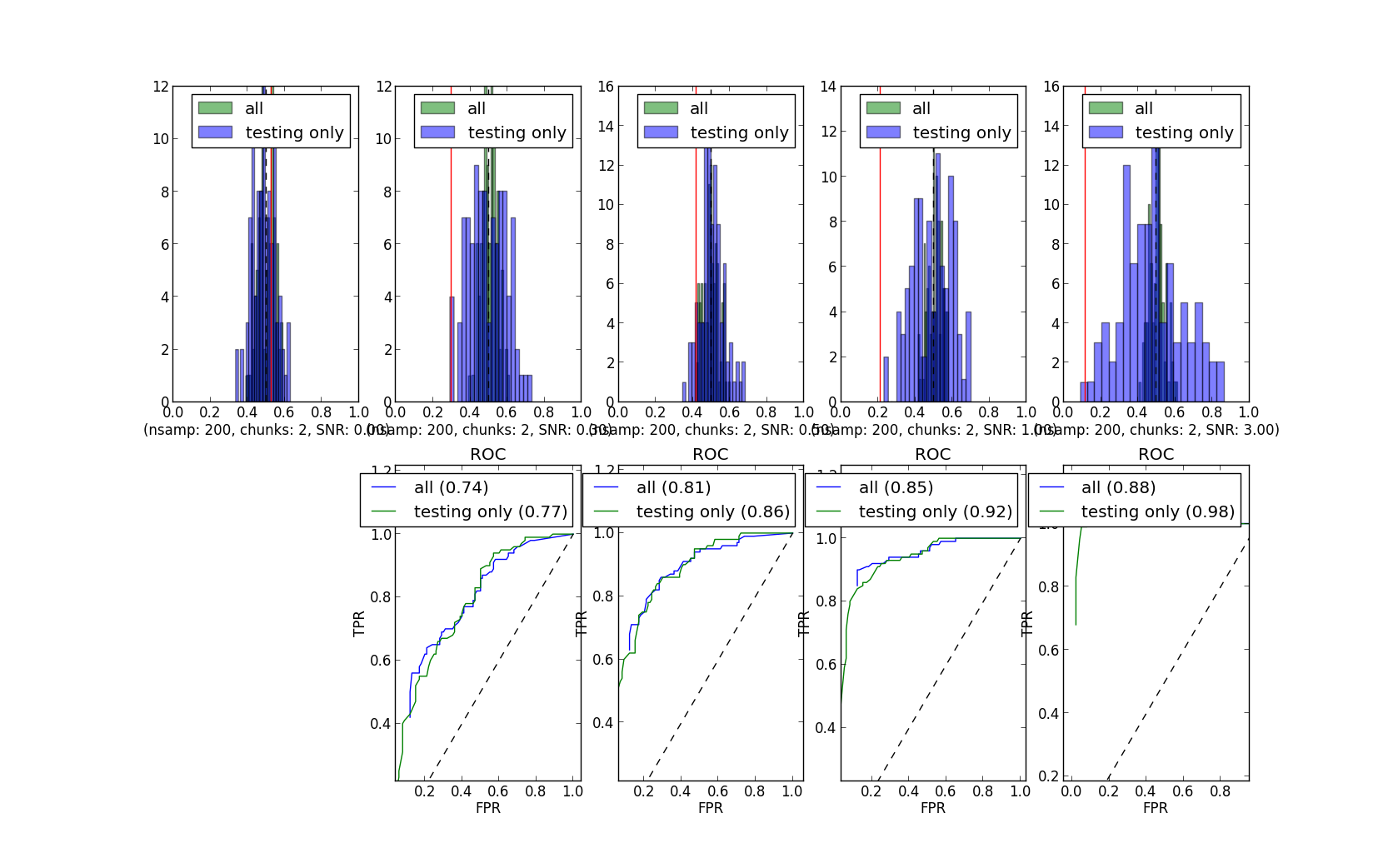
This post could also be titled: "how you simulate the data really matters". In my previous post about changing the difference between the two classes (how much information, how easy to classify) I found that fairly large changes to the "bias" changed the accuracy (and so p-values) drastically, but not the null distributions.

Changing how I generated the simulated data causes the null distributions to change a lot as the difference between the classes increases. These simulations are the same as the previous set (same seeds, number of examples, cross-validation schemes, relabeling schemes, linear svms, etc), except for how the simulated data was generated.

In these examples, higher "snr" corresponds to easier classification (so the dark lines have more signal). When permuting the training set labels only the null distribution changes dramatically (and very strangely), becoming wider as the snr increases.


What is the difference?

In my original simulations the variance increased minimally with signal. I made the values for one voxel with the R code
tbl[,i] <- c(rnorm(40, mean=-0.15, sd=1), rnorm(40, mean=0.15, sd=1));
which generates 40 entries at random from a standard normal distribution with standard deviation 1 and mean -0.15 to be the 40 values for that voxel in class A, and 40 entries from a normal distribution with standard deviation 1 and mean 0.15 to be the values for that voxel in class B. (This is for 4 runs with 10 examples in each run, and a "bias" of 0.15.)

I set up the simulation for this post to mimic the description of the pyMVPA normal_feature_dataset function, which was used in the simulations on the pyMVPA message list. I kept the parameters similar to my previous simulation (all voxels have signal), but used this R code to generate data for one voxel:
temp.vox <- rnorm(40, mean=0, sd=1);
temp.vox2 <- temp.vox / pymvpa.snr; 

temp.vox <- c(temp.vox, temp.vox2);
tbl[,i] <- temp.vox / max(abs(temp.vox));

Where pymvpa.snr is 0.3, 3, 10, or 30. In words, I choose 40 entries from a standard normal distribution with standard deviation 1 and mean 0 to be the 40 values for that voxel in class A. I then divided each of the 40 values by the signal-to-noise ratio (e.g. 0.3), and set those values for class B. Finally, I divided each value by the largest absolute value of any of the 80 values.

Dividing by a constant (the signal-to-noise) makes fairly large differences in the variance of the A and B samples as the constant changes, even after normalization, and I think that might be driving the "widening" of the null distribution with increased signal, and certainly makes large differences to the null distributions.

So ...

If such effects of how datasets are simulated are widespread, we'll have to be much more careful in explaining how simulations were conducted, and perhaps try to decide on a standard. Which methods are actually closest to fMRI data? Or can we even determine a general case, given how much fMRI preprocessing can vary?

UPDATE: this is not an accurate description of the normal_feature_dataset function. See this post for details.

Wednesday, September 19, 2012

pyMVPA searchlight shape: solved

Michael Hanke posted further description of the pyMVPA searchlight: it is the same as the Princeton MVPA toolbox searchlight I described earlier.

As Michael points out, it is possible to define other searchlight shapes in pyMVPA; this is the default for a sphere, not the sole option.

Tuesday, September 11, 2012

pyMVPA searchlight shapes

Michael Hanke listed the number of voxels for different searchlight radii in pyMVPA. He also wrote that pyMVPA considers neighboring voxels to be those that share two edges (i.e., a face).

Here's a diagram of following the faces-touching rule. The center voxel is black, the one-voxel radius surrounds red, the two-voxel radius surrounds purple, and the three-voxel radius surrounds blue.
This gives 1 + 9 + 21 + 24 + 21 + 9 + 1 = 86 surrounding voxels for the three-voxel radius.

But Michael wrote that a three-voxel radius searchlight in pyMVPA has 123 voxels (counting the center). If so, at left is how I could come by that count: 13 + 28 + 40 + 28 + 13 = 122.

This shape is not quite symmetrical: there are four voxels to the left, right, front, and back of the center voxel but only two above and below.

Anyone know if this is what pyMVPA does?

UPDATE: Neither of these sketches is correct, see pyMVPA searchlight: solved.