DMCC13benchmark: public again

Apologies: I've had to temporarily delete DMCC13benchmark from OpenNeuro. We plan to upload a new version ASAP. The images and associated data in the new version will be the same, and I will keep the same dataset name.

The problem was with the subject ID codes: some of the DMCC participants were members of the Young Adult HCP, and we released DMCC13benchmark with those HCP ID codes. In consultation with members of the HCP we decided that it would be most appropriate to release data with unique ID codes instead. The subject key (linking the subject IDs released on openneuro to the actual HCP ID codes) is available via the HCP ConnectomeDatabase for people who have accepted the HCP data use terms (ConnectomeDB00026, titled "DMCC (Dual Mechanisms of Cognitive Control) subject key").

Again, I apologize for any inconvenience. We are working to upload a corrected version of DMCC13benchmark soon. Please contact me with questions or if you need something sooner; I will add links to this post when DMCC13benchmark is again public.

UPDATE 4 January 2021: The corrected version of DMCC13benchmark is now available as openneuro dataset ds003452, doi: 10.18112/openneuro.ds003452.v1.0.1. We ask anyone using the dataset to use this version (all subject IDs starting with "f") rather than the previous. Every file should be identical between the versions, excepting the subject IDs.

I again apologize for any inconvenience this change may have caused you, and urge you to contact me with any questions or concerns.

 

comparing fMRIPrep and HCP Pipelines: Resting state blinded matching

The previous post has a bit of a literature review and my initial thoughts on how to compare resting state preprocessing pipeline output. We ended up trying something a bit different, which I will describe here. I actually think this turned out fairly well for our purposes, and has given me sufficient confidence that the two pipelines have qualitatively similar output.

First, the question. As described in previous (task-centric) posts, we began preprocessing the DMCC dataset with the HCP pipelines, followed by code adapted from Josh Siegel (2016) for the resting state runs. We are now switching to fmriprep for preprocessing, followed by the xcpEngine (fc-36p) for resting state runs. [xcp only supports volumes for now, so we used the HCP pipeline volumes as well.] Our fundamental concern is the impact of this processing switch: do the two pipelines give the "same" results? We could design clear benchmark tests for the task runs, but how to test the resting state analysis output is much less clear, so I settled on a qualitative test.

We're using the same DMCC13benchmark dataset as in the task comparisons, which has 13 subjects. Processing each with both pipelines gives 26 total functional connectivity matrices. Plotting the two matrices side-by-side for each person (file linked below) makes similarities easy to spot: it looks like the two pipelines made similar matrices. But we are very good at spotting similarities in paired images; are they actually similar?

The test: would blinded observers match up the 26 matrices by person (pairing the two matrices for each subject) or by something else (such as pipeline)? If observers can match most of the matrices by person, we have reason to think that the two pipelines are really producing similar output. (Side note: these sorts of tests are sometimes called Visual Statistical Inference and can work well for hard-to-quantify differences.)

For details, here's a functional connectivity matrix for one of the DMCC13benchmark subjects. There are 400 rows and columns in the matrix, since these were run within the Schaefer (2018) 400-parcels 7-network ordering parcellation. This parcellation spans both hemispheres, the first 200 on left, second 200 right. Both hemispheres are in the matrix figures (labeled and separated by black lines). The number of parcels in each network is not perfectly matched between hemispheres, so only the quadrants along the diagonal have square networks. The dotted lines separate the 7 networks: Visual, SomMot, DorsAttn, SalVentAttn, Limbic, Cont, Default (ordering and labels from Schaefer (2018)). Fisher r-to-z transformed correlations are plotted, with the color range from -1.9 (darkest blue) to 1.9 (darkest red); 0 is white.
 
Interested in trying to match the matrices yourself? This pdf has the matrices in a random order, labeled with letters. I encourage you to print the pdf , cut the matrices apart, then try to pair them into the 13 people (we started our tests with the matrices in this alphabetical order). I didn't use a set instructional script or time limit, but encouraged people not to spend more than 15-20 minutes or so, and explained the aim similarly to this post. If you do try it, please note in the comments/email me your pairings or number correct (as well as your strategy and previous familiarity with these sorts of matrices) and I'll update the tally. The answers are listed on the last page of this pdf and below the fold on this post.

Several of us had looked at the matrices for each person side-by-side before trying the blind matching, and on that basis thought that it would be much easier to pair the people than it actually was. Matching wasn't impossible, though: one lab members successfully matched 9 of the 13 people (the most so far). At the low end, two other lab members only successfully matched 2 of the 13 people; three members matched 4, one 5, one 7, and one 8.

That it was possible for anyone to match the matrices for most participants reassures me that they are indeed more similar by person than pipeline: the two pipelines are producing qualitatively similar matrices when given the same input data. For our purposes, I find this sufficient: we were not attempting to determine if one version is "better" than the other, just if they are comparable.

What do you think? Agree that this "test" suggests similarity, or would you like to see something else? pdfs with the matrices blinded and not are linked here; let me know if you're interested in the underlying numbers or plotting code and I can share that as well; unpreprocessed images are already on OpenNeuro as DMCC13benchmark.

Assigned pairings (accurate and not) after the jump.

UPDATE 3 December 2019: Correlating the functional connectivity matrices is now described in a separate post. 

UPDATE 4 January 2021: Corrected DMCC13benchmark openneuro links.

comparing fMRIPrep and HCP Pipelines: Resting state matrix correlation

In the previous post I described comparing resting state pipelines by asking blinded people to match functional connectivity matrices by participant. As described in that post, while no one correctly matched all matrices (i.e., pairing up the hcp-Siegel and fmriprep-xcp versions for the 13 people in DMCC13benchmark), most correctly matched many of them, reassuring me that the two pipelines are producing qualitatively similar functional connectivity matrices.

In this post I show the results of correlating the functional connectivity matrices, on the suggestion of Max Bertolero (@max_bertolero, thanks!). Specifically, I turned the lower triangles of each connectivity matrix into a vector then correlated them pairwise. (In other words, "unwrapping" each functional connectivity matrix into a vector then calculating all possible pairwise correlations between the 26 vectors.)

The results are in the figure below. To walk you through it: participants are along the x-axis, matrix-to-matrix correlations  on the y-axis. Each person is given a unique plotting symbol, which is shown in black. The first column is for person 150423, whose plotting symbol is a circle. The correlation of 150423's hcp-Siegel and fmriprep-xcp matrices is about 0.75 (location of the black circle). The four colored sets of symbols are the correlation of 150423's hcp or fmriprep matrix with everyone else's hcp or fmriprep matrices, as listed along the top. For example, the bright blue column is listed as "hcp w/others' fp", and the highest symbol is a plus. Looking at the black symbols, the plus sign is 171330, so this means that the correlation of 150423's hcp-Siegel matrix with 171330's fmriprep-xcp matrix is about 0.63.

There are several interesting parts of the figure. First, the dark blue and dark red points tend to be a bit higher than the bright blue and pink: matrices derived from the same pipeline tend to have higher correlation than those from different pipelines, even from different people.

Next, most people's fmriprep and hcp matrices are more correlated than either are to anyone else's - the black symbols are usually above all of the colored ones. This is not the case for 3 people: 178950, DMCC8033964, and DMCC9478705. 203418 is also interesting, since their self-correlation is a bit lower than most, but still higher than the correlation with all the others.

Finally, I compared the impressions from this graph with those from the blinded matching (summarized in the table below), and it came out fairly consistently, particularly for the hardest to match pairs: No one correctly matched 178950 or DMCC9478705's matrices, two of the people just listed as having their self-correlations in the midst of the others. Only one person correctly matched the third (DMCC8033964).

While the hardest-to-match pairs are easy to see in this graph, the ones most often correctly matched are more difficult to predict. For example, from the height of the self-correlation and distance to the other points I'd predict that 171330 and 393550 would be relatively hard to pair, but they were the most often correctly matched. 203418 has the fourth-lowest self-correlation, but was correctly matched by more than half the testers.

Note: the "correct matches" column is how many of the 9 people doing the blinded matching test correctly matched the person's matrices.

subject ID	correct pairing (hcp, fmriprep)	correlation of this person’s matrices	correct matches
150423	h,q	0.7518	4
155938	v,i	0.7256	6
171330	l,y	0.7643	4
178950	b,r	0.6069	0
203418	x,d	0.651	5
346945	w,j	0.7553	4
393550	u,n	0.7772	7
601127	c,m	0.7152	1
849971	k,t	0.7269	1
DMCC5775387	s,f	0.767	6
DMCC6705371	a,p	0.733	6
DMCC8033964	g,z	0.5938	1
DMCC9478705	o,e	0.5428	0

Together, both the blinded matching and correlation results reassure me that the two pipelines are giving qualitatively similar matrices, but clearly not identical, nor equally similar for all of the test people.


UPDATE 4 December 2019: Checking further, missings have a sensible impact on these results. These functional connectivity matrices were not calculated from the DMCC baseline session only (which are the runs included in DMCC13benchmark), but rather by concatenating all resting state runs for the person in the scanning wave. Concatenating gives 30 minutes of resting state total without missings or censoring.

Two subjects had missing resting state runs: DMCC8033964 is missing one (25 minutes total instead of 30), and DMCC9478705 is missing two (20 minutes). These are two of the lowest-correlation people, which is consistent with the expectation that longer scans make more stable functional connectivity matrices. It looks like the two pipelines diverge more when there's fewer input images, which isn't too surprising. 178950 didn't have missing runs but perhaps had more censoring or something; I don't immediately know how to extract those numbers from the output but expect the pipelines to vary in many details.

UPDATE 4 January 2021: Corrected DMCC13benchmark openneuro links.

comparing fMRIPrep and HCP Pipelines: with version 1.3.2

We've been working on preparing to switch our DMCC preprocessing pipelines over to fMRIPrep. For the resting state component we decided to use the XCP system, which works well with fMRIPrep-preprocessed datasets ... but (as of April 2019) requires fMRIPrep version 1.3.2, not the version 1.1.7 we'd used in our preprocessing comparisons (since that was the current version when we began). A quick check showed that fMRIPrep version 1.3.2 and 1.1.7 produced similar - but not identical - images, so we reran the comparisons, using fMRIPrep version 1.3.2.

As we'd hope, the differences in the preprocessed images and GLM results between fMRIPrep version 1.1.7 and 1.3.2 are very small, much smaller than between either fMRIPrep version and the HCP pipeline, at both the single subject and group level. The conclusions in my previous summary post apply to the 1.3.2 results as well. Here I'll show some group results to parallel the previous summary; contact me if you'd like more of the results, more detail, or the underlying data.

First, the same 20 Schaefer parcels passed the threshold of having t > 1 (uncorrected) in all four tasks and preprocessing combinations when the fp132 (fMRIPrep version 1.3.2) results were substituted for the previous 1.1.7 results (compare with here and here):

This is not surprising, given the extremely similar GLM results for each person between the two fMRIPrep versions. Using these 20 parcels, I made some scatterplots to show the comparison in coefficients between the various preprocessing styles (the ones for HCP and fMRIPrep ("fp") are the same as in the previous summary, just with tasks overplotted; see that post for more explanation). Note that in these plots "fp132" is fMRIPrep version 1.3.2 and "fp" or "fMRIPrep" is version 1.1.7.

It is clear that the tightest correlations are between the two versions of fMRIPrep preprocessing, surface to surface and volume to volume ("fp132 vs. fMRIPrep"). The plots comparing "HCP vs. fMRIPrep" (1.1.7) and "HCP vs. fp132" are similar, as are the "Volume vs. Surface" plots within each fMRIPrep version.

I also set up mixed models as before, adding the fMRIPrep 1.3.2 results. The contrasts below are from a model including all four tasks, the 20 parcels, and the 13 test people, only estimating the effect of preprocessing combination on the parameter difference. I highlighted the interesting contrasts: red are volume vs. surface within each pipeline (surface better for both fMRIPrep versions); blue show that the two fMRIPrep versions were not different; green shows that the surface estimates were higher with either fMRIPrep than HCP, and volume estimates marginally higher.

So, we're still "full steam ahead" with fMRIPrep. I don't know which part of the fMRIPrep pipeline changed between 1.1.7 and 1.3.2 to make our results slightly different, but the differences don't change the interpretation of the comparisons.

UPDATE 6 September 2019: The dataset (raw and preprocessed images) we used for these comparisons is now on openneuro, called DMCC13benchmark.

UPDATE 4 January 2021: Corrected DMCC13benchmark openneuro links.

DMCC GLMs: afni TENTzero, knots, and HDR curves, #1

One of the things we've been busy with during the pandemic-induced data collection pause is reviewing  the DMCC (Dual Mechanisms of Cognitive Control; more descriptions here and here) project GLMs: did we set them up and are we interpreting them optimally? 

We decided that the models were not quite right, and are rerunning all of them. This post (and its successors) will describe how the original GLMs were specified, why we thought a change was needed, what the change is, and how the new results look. The posts are intended to summarize and clarify the logic and process for myself, but also for others, as I believe many people find modeling BOLD responses (here, with afni 3dDeconvolve TENTs) confusing.

 

I won't just start explaining the DMCC GLMs however, because they're complex: the DMCC has a mixed design (task trials embedded in long blocks), and we're estimating both event-related ("transient") and block-related ("sustained") responses. If you're not familiar with them, Petersen and Dubis (2012) review mixed block/event fMRI designs, and Figure 1 from Visscher, et. al (2003) (left) illustrates the idea. In addition to the event and block regressors we have "blockONandOFF" regressors in the DMCC, which are intended to capture the transition between the control and task periods (see Dosenbach et. al (2006)).

We fit many separate GLMs for the DMCC, some as controls and others to capture effects of interest. For these posts I'll describe one of the control analyses (the "ONs") to make it a bit more tractable. The ON GLMs include all three effect types (event (transient), block (sustained), blockONandOFF (block start and stop)), but do not distinguish between the trial types; all trials (events) are given the same label ("on"). The ON GLMs are a positive control; they should show areas with changes in activation between task and rest (30 seconds of fixation cross before and after task blocks). For example, there should be positive, HRF-type responses in visual areas, because all of our task trials include visual stimuli.

Below is an example of the estimated responses from our original ONs GLMs (generated by R knitr code similar to this). The GLMs were fit for every voxel individually, then averaged within the Schaefer, et al. (2018) parcels (400x7 version); these are results for four visual parcels and volumetric preprocessing. These are (robust) mean and SEM over 13 participants (DMCC13benchmark). The results have multiple columns both because there are four DMCC tasks (Axcpt (AX-CPT), Cuedts (Cued task-switching), Stern (Sternberg working memory), and Stroop (color-word variant)), and because of the mixed design, so we generate estimates for both event/transient (lines) and sustained (blue bars) effects (blockONandOFF are not included here).

The line graphs show the modeled response at each time point ("knot"). Note that the duration (and so number of estimated knots) for each task varies; e.g., Stroop has the shortest tasks and Stern the longest. (We set the modeled response to trial length + 14 seconds.)

The double-peak response shape for Axcpt, Cuedts, and Stern is expected, as the trials have two stimuli slides separated by a 4 second ITI; the Stroop response should resemble a canonical HRF since each trial has a single stimulus and is short. The task timing and some sample trials are shown below (this is  Figure 1 in a preprint (accepted version) which has much more task detail; see also the DMCC55B description). 

So far, so good: the estimated responses for each task have a sensible shape, reflecting both the HRF and task timing. But what exactly is along the x-axis for the curves? And how did we fit these GLMs, and then decide to change them a bit? ... stay tuned.

later posts in this series: #2

UPDATE 4 January 2021: Corrected DMCC13benchmark openneuro links.

an introduction to DMCC55B

It's hard to believe this is my first post of 2021! I've done a few updates to existing posts during the last few months, but not the detailed new ones I've been planning; hopefully this will be the first of a small "flurry" of new posts.

Here, I'm happy to announce the first big public release of Dual Mechanisms of Cognitive Control (DMCC) project data, "DMCC55B", together with a detailed description and example analyses. We've previously released smaller parts of the DMCC (DMCC13benchmark), which has been very useful for methods exploration, but isn't really enough data for detailed analysis of the task-related activity or individual differences. A wide range of analyses are possible with DMCC55B, and we hope the documentation both clear and detailed enough to make its use practical.

A few highlights: DMCC55B is data from 55 unrelated young adults. Each participant performed four cognitive control tasks (Stroop, AX-CPT, Cued Task-Switching, and Sternberg Working Memory) while undergoing moderately high-resolution fMRI scanning (MB4, 2.4 mm isotropic voxels, 1.2 s TR). Two runs of each task (one with AP encoding, the other PA), of approximately 12 minutes each (about 1.5 hours of task fMRI per person). There are also scores for the participants on 28 state and trait self-report questionnaires, as well as finger photoplethysmograph and respiration belt recordings collected during scanning.

This manuscript is intended to be the practical introduction to DMCC55B, providing details such as e.g., the file format of questionnaire data, the order in which task stimuli were presented, fMRI preprocessing (fmriprep output is included), and how Stroop responses were collected and scored. The manuscript also contains links and references to materials used for the main DMCC project (e.g., eprime task presentation scripts, code to extract reaction times from the Stroop audio recordings), which may be of interest or use to others in some cases, but likely only in a few specialized instances. A separate manuscript (preprint; accepted version) describes the wider DMCC project, including the theoretical basis for the task design. If some information is confusing or missing, please let me know!

Last, but most definitely not least, I want to highlight the "supplemental" accompanying DMCC55B. This designed to perform and summarize some standard behavioral and quality control analyses, with the intention of the files serving both as an introduction to working with DMCC data (e.g., how do I obtain the onset time of all AX trials?) and analysis tutorials (e.g., of a parcel-wise classification MVPA with surface data). Currently, the best introduction to this material is in the DMCC55B manuscript and the files themselves. The supplemental files are primarily knitr (R and LaTeX); they call afni functions (e.g., 3dTstat) directly when needed, and are entirely "untidy" base R, including base R graphics. (The last bit refers to the different "flavors" of R programming; I only rarely have need to visit the Tidyverse.)

 

 UPDATE 13 September 2021: Added a link to the published version of the DMCC overview manuscript.

comparing fMRIPrep and HCP Pipelines: introduction

This is the first in a series of posts describing a set of comparisons we've done between fMRIPrep and the HCP Pipelines: if the same task fMRI dataset is run through both pipelines, extracting surfaces and volumes from each, how do the eventual GLM results compare?

These sorts of comparisons are conceptually easy but tricky to design and time-consuming to complete. I submitted this as a poster for OHBM 2019, we will likely write this up as a paper, and  plan to release the code and images. But these blog posts are a start, and feedback is most welcome. Let me know if you want additional details or files and I can try to get them to you sooner than later.

roadmap

• This post describes the dataset, preprocessing, tasks, GLMs, and parcellation (for ROIs). 
• The next post(s) will show the output of the two pipelines, as motion regressors, QC metrics, and images.
• Then posts will describe and compare the GLM statistics calculated from each set of images: full-brain images, parcel-wise curves, by target knots in the parcels, and a subset of the parcels. 

The final post also has some summary thoughts. An UPDATE (24 April 2019) describes the same analyses run with fMRIPrep version 1.3.2.

dataset

I am particularly interested in how the preprocessing would affect the statistics for the Dual Mechanisms of Cognitive Control (DMCC) project since that's the project I'm most involved with. I've previously shown bits from this dataset and described the acquisition parameters; briefly, each DMCC scanning session includes two runs each of four cognitive control tasks (AX-CPT, Cued task-switching, Sternberg, and Stroop). Task runs were each approximately 12 minutes, alternating AP/PA. All scanning was with a 3T SIEMENS Prisma scanner with a 32 channel head coil, 2.4 mm isotropic voxels, TR = 1.2 s, and an MB4 CMRR sequence.

The DMCC is a big dataset (currently around 80 people with at least 3 scanning sessions, and we're not done). To keep the preprocessing comparisons tractable I picked just 13 of the participants to include, requiring that they have complete Baseline session data (two runs of each of the four tasks), be unrelated, have acceptable movement (a qualitative judgement), and have visible motor activity in their single-subject Buttons GLMs (with HCP Pipeline preprocessing). This last is an effort for an unbiased QC estimate: in three of our tasks the participants push a response button, so GLMs using these button-pushes as the only events of interest (ignoring all of the cognitive conditions) should show motor activation if the signal quality is acceptable. I used the volumetric HCP Pipeline preprocessing for screening because that's what we've been using (and so have results for all people); that may introduce a bit of bias (favoring people that did well with the volumetric HCP Pipelines).

pipelines, GLMs, and parcels

These analyses use version 3.17.0 of the HCP Pipelines (adapted several years ago for the DMCC acquisitions) and fMRIPrep version 1.1.7; each pipeline began with the same DICOM images.

The same GLMs (event onsets, model types, etc.) were run on the images from each version (surface, volume) of each pipeline; all with AFNI. The "standard" DMCC GLMs are not particularly simple because the task runs are mixed (block and event), and we're fitting GLMs to model both "sustained" (block) and event-related activity. The GLMs use 3dDeconvolve and 3dREMLfit, with TENTzero (FIR-type) for the events (one knot for two TRs). Most of the GLM model parameters were dictated by the experimental design, but tweaking (e.g., how long to make the TENT knots, whether to include regressors for the block onsets and offsets) was done with the HCP pipeline preprocessed images.

To keep these preprocessing comparisons tractable at the GLM level, we only included Baseline session images, and focused on contrasting high and low cognitive control. Which trials correspond to high and low cognitive control varies across the four tasks, and we don't expect identical levels of difficulty or brain activity in the tasks. Regardless, high vs. low cognitive control conditions gives a fairly "apples to apples" basis, and is a reasonably strong effect.

Another complication for preprocessing comparisons is working out the anatomical correspondence: every voxel does not have a single vertex in the surface representation (and each vertex doesn't match a single voxel). While we had both the fMRIPrep and HCP Pipelines output MNI-normalized volumes (so volume-to-volume voxel-level correspondence), the two pipelines use different surface meshes (fsaverage5 vs. HCP), so there isn't an exact match between the vertices (see this thread, for example).

For these comparisons I deal with corresponding across the output formats by making qualitative assessments (e.g., if this GLM output statistic is thresholded the same, do the same areas tend to show up in the volumes and surfaces?), but more practically by summarizing the statistics within anatomic parcels. The parcellation from (Schaefer et al. 2017) is ideal for this: they released it in volume (MNI) and surface (both fsaverage5 and HCP) formats.We used the 400-area version here, allowing direct comparisons: a mean of parcel #6 can be computed in all four output images (HCP volume, HCP surface, fMRIPrep volume, fMRIPrep surface). The number of voxels or vertices making up each parcel varies between the volume and surfaces, of course.


UPDATE 10 January 2019: Here's the command actually used to run fMRIPrep; thanks Mitch Jeffers!
singularity run \
--cleanenv \
-B ${MOUNT}:/tmp \
/home/ccp_hcp/fmriprep/SingularityImages/fmriprep-1.1.7.simg \
--fs-license-file /tmp/.license/freesurfer/license.txt \
-w /tmp \
/tmp/${INPUT} /tmp/${OUTPUT} \
participant --participant_label ${SUBJECT} \
--output-space fsaverage5 \
-n-cpus 16 --omp-nthreads 4 \
--mem-mb 64000 -vvvv \
--use-plugin /tmp/plugin.yml


UPDATE 6 September 2019: The raw and preprocessed images of the dataset we used for these comparisons is now on openneuro, called DMCC13benchmark. 

UPDATE 4 January 2021: Corrected DMCC13benchmark openneuro links.

DMCC GLMs: afni TENTzero, knots, and HDR curves, #2

This post is the second in a series, which begins with this post. In that first post I included examples of the estimated HDR curves for a positive control analysis, one of which is copied here for reference. 

What are the axis labels for the estimated HDR curves? How did we generate them? What made us think about changing them? 

At the first level the (curve) axis label question has a short answer: y-axes are average (across subjects) beta coefficient estimates, x-axes are knots. But this answer leads to another question: how do knots translate into time? Answering this question is more involved, because we can't translate knots to time without knowing both the TR and the afni 3dDeconvolve command. The TR is easy: 1.2 seconds. Listing the relevant afni commands is also easy:

3dDeconvolve \  
 -local_times \  
 -x1D_stop \  
 -GOFORIT 5 \  
 -input 'lpi_scale_blur4_tfMRI_AxcptBas1_AP.nii.gz lpi_scale_blur4_tfMRI_AxcptBas2_PA.nii.gz' \  
 -polort A \  
 -float \  
 -censor movregs_FD_mask.txt \  
 -num_stimts 3 \  
 -stim_times_AM1 1 f1031ax_Axcpt_baseline_block.txt 'dmBLOCK(1)' -stim_label 1 ON_BLOCKS \  
 -stim_times 2 f1031ax_Axcpt_baseline_blockONandOFF.txt 'TENTzero(0,16.8,8)' -stim_label 2 ON_blockONandOFF \  
 -stim_times 3 f1031ax_Axcpt_baseline_allTrials.txt 'TENTzero(0,21.6,10)' -stim_label 3 ON_TRIALS \  
 -ortvec motion_demean_baseline.1D movregs \  
 -x1D X.xmat.1D \  
 -xjpeg X.jpg \  
 -nobucket  
 
3dREMLfit \
 -matrix X.xmat.1D \
 -GOFORIT 5 \
 -input 'lpi_scale_blur4_tfMRI_AxcptBas1_AP.nii.gz lpi_scale_blur4_tfMRI_AxcptBas2_PA.nii.gz' \
 -Rvar stats_var_f1031ax_REML.nii.gz \
 -Rbuck STATS_f1031ax_REML.nii.gz \
 -fout \
 -tout \
 -nobout \
 -verb

Unpacking these commands is not so easy, but I will try to do so here for the most relevant parts; please comment if you spot anything not quite correct in my explanation.

First, the above commands are for the Axcpt task, baseline session, subject f1031ax (aside: their data, including the event timing text files named above, is in DMCC13benchmark). The 3dDeconvolve command has the part describing the knots and HDR estimation; I included the 3dREMLfit call for completeness, because the plotted estimates are from the Coef sub-bricks of the STATS image (produced by -Rbuck).

Since this is a control GLM in which all trials are given the same label there are only three stimulus time series: BLOCKS, blockONandOFF, and TRIALS (this is a mixed design; see introduction). The TRIALS part is what generates the estimated HDR curves plotted above, as defined by TENTzero(0,21.6,10).

We chose TENTzero instead of TENT for the HDR estimation because we do not expect anticipatory activity (the trial responses should start at zero) in this task. (see afni message board, e.g., here and here) To include the full response we decided to model the trial duration plus at least 14 seconds (not "exactly" 14 seconds because we want the durations to be a multiple of the TENT duration). My understanding is that it's not a problem if more time than needed is included in the duration; if too long the last few knots should just approximate zero. I doubt you'd often want to use a duration much shorter than that of the canonical HRF (there's probably some case when that would be useful, but for the DMCC we want to model the entire response).

From the AFNI 3dDeconvolve help: 

'TENT(b,c,n)': n parameter tent function expansion from times b..c after stimulus time [piecewise linear] [n must be at least 2; time step is (c-b)/(n-1)]

 

You can also use 'TENTzero' and 'CSPLINzero',which means to eliminate the first and last basis functions from each set. The effect of these omissions is to force the deconvolved HRF to be zero at t=b and t=c (to start and and end at zero response). With these 'zero' response models, there are n-2 parameters (thus for 'TENTzero', n must be at least 3).

The first TENTzero parameter is straightforward: b=0 to start at the event onset.

For the trial duration (c), we need to do some calculations. Here, the example is the DMCC Axcpt task, which has a trial duration of 5.9 seconds, so the modeled duration should be at least 14 + 5.9 = 19.9 seconds. That's not the middle value in the TENTzero command, though.

For these first analyses we decided to have the TENTs span two TRs (1.2 * 2 = 2.4 seconds), in the (mostly) mistaken hope it would improve our signal/noise, and also to make the file sizes and GLM estimation speeds more manageable (which it does). Thus, c=21.6, the shortest multiple of our desired TENT duration greater than the modeled duration (19.9/2.4 = 8.29, rounded up to 9; 9*2.4 = 21.6). 

Figuring out n requires a bit of mind bending but less calculation; I think the slide below (#5 in afni06_decon.pdf) helps: in tent function deconvolution, the n basis functions are divided into n-1 intervals. In the above calculations I rounded 8.29 up to 9; we want to model 9 intervals (of 2.4 s each). Thus,  n = 10 basis functions gives us the needed n-1 = 9 intervals.

Recall that since we're using TENTzero, the first and last tent functions are eliminated. Thus, having n=10 means that we will get 10-2=8 beta coefficients ("knots") out of the GLM. These, finally, are the x-axes in the estimated GLM curves above: the knots at which the HDR estimates are made, of which there are 8 for Axcpt. 

(Aside: 0-based afni can make some confusion for those of us more accustomed to 1-based systems, especially with TENTzero. The top plots put the value labeled as #0_Coef at 1; a point is added at 0=0 since TENTzero sets the curves to start at zero. I could also have added a zero for the last knot (9, for this Axcpt example), but did not.)

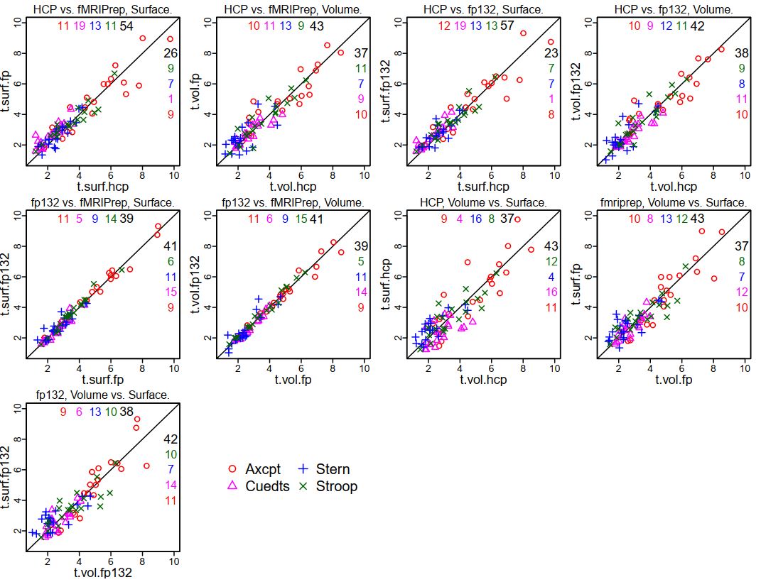
These GLMs seem to be working fine, producing sensible HDR estimates. We've been using these results in many analyses (multiple lab members with papers in preparation!), including the fMRIprep and HCP pipeline comparisons described in previous posts. We became curious, though, if we could set the knot duration to the TR, rather than twice the TR (as done here): would the estimated HDR then follow the trial timing even more precisely? In the next posts(s) I'll describe how we changed the GLMs to have the knot duration match the TR, and a (hopefully interesting) hiccup we had along the way.

UPDATE 4 January 2021: Corrected DMCC13benchmark openneuro links.

observation: variability from running fmriprep multiple times

UPDATE 13 May 2020: I'm now quite sure that the high variability wasn't due to the multiple fmriprep runs, but rather the way I picked the training/testing examples. I'm leaving this post here, but put most of it "below the fold" since my initial interpretation was incorrect. I will eventually release code and more details.

UPDATE 24 April 2020: I realized that there was at least one other possible big contributing factor to the difference between the runs: randomness in how I chose the not-button examples. I'll fix this and see what happens to the SVM results. I previously found extremely similar GLM results between fmriprep versions 1.1.2 and 1.3.2, so the variability here is very possibly only from my randomness in setting up the classification.