overlaying in Connectome Workbench 1.4.2

This post answers a question posted on my Workbench introductory tutorial: Rui asked how to visualize the common regions for two overlays. I've found two ways of viewing overlap.

The first is to reduce the Opacity (circled in red) of the top-most Layer. In this screen capture I have a blueish ROI on top of a yellow one. (I scribbled the colors over their corresponding rows in the Layers toolbox; blue is listed above - over - the yellow. Click the Layers On and off if you're not sure which is which.) Compare the appearance of the ROIs when the Opacity is set to 1.0 for both (left) versus 0.7 for the top (blue, right): the borders of both ROIs are visible on the right side, and the blue is less opaque all over (not just in the area that overlaps).

The second method is to set one (or both) ROIs to Outline (border) mode. Here, I set the top (blue) ROI to "Outline Only" in the Overlay and Map Settings dialog box (click the little wrench button to bring up the dialog).

Getting started with Connectome Workbench 1.4.2

Here is an updated version of my introductory tutorial for the Connectome Workbench, written for Workbench 1.4.2. This new version of Workbench has some nice features (only a few of which are described here!), so I suggest you try this one rather than a previous version. I have a few other posts on Workbench and HCP-related topics, mostly linked from the "Connectome Workbench: 1st steps" post.

downloading the program

Connectome Workbench has versions for Windows, Mac OS, and Linux; just click the download link for your OS (Linux types can also install Workbench via NeuroDebian).

On Windows and Mac you don't "install" Workbench, but just unzip the download then double-click the executable. On my windows box I put the download into d:\Workbench\, unzipped it, and got a bunch of subdirectories. Navigate through until you find wb_view; in my case it's at D:\Workbench\workbench-windows64-v1.4.2\bin_windows64\wb_view.exe. Double-click wb_view to start the program. If you don't want to navigate to this directory each time to start Workbench, make a shortcut to wb_view.exe and put it on your desktop or in a handy menu.

Aside: wb_command.exe is in the same directory as wb_view.exe. wb_command.exe is not a GUI program (nothing much will happen if you double-click it!), but is useful for various functions; see this post and this documentation for more.

getting images to plot

Workbench doesn't come with any images, so this tutorial will use ones from my knitr tutorials, available at https://osf.io/w7zkc/. Download all of the files under "knitr tutorials", the "surface (GIFTI) brain plotting" and "volumetric (NIfTI) brain plotting" subdirectories. (The .rnw files should be kept in separate directories if you're going to compile the knitr tutorials.)

Aside: Only the files from the osf site are needed for this tutorial, but you will likely want more anatomic underlays than these. I suggest underlays from the HCP S1200 release for volumetric (MNI) and fsLR surfaces; I converted the fsaverage5 surfaces from our local FreeSurfer installation, but FreeSurfer provides many more than the pair I put into osf.

seeing blank brains

Open the Workbench GUI (e.g., by double-clicking wb_view.exe). A command window will open (just ignore it), as well as a interactive box prompting you to open a spec or scene file. Click the Skip button to load the main program. Note: spec and scene files are very useful, and a big reason to use Workbench, because they let you save collections of images and visualizations, which can save a massive amount of time. I won't cover them in this tutorial, though.

Since we skipped loading anything, Workbench opens with a blank screen. We want to first open images to use as underlays: a NIfTI volumetric underlay to plot volumetric blobs on, and GIFTI surface files to plot surface blobs on (see this post for a bit more about file types).

Select File -> Open File from the top menus to open a standard file selection dialog. Navigate to where you put the images from "surface (GIFTI) brain plotting", and change the Files of type drop-down to "Surface Files (*.surf.gii)", then select and open the four fsaverage5 .surf.gii files (two hemispheres * two inflations). Open the Open File dialog again, navigate to where you put the files from "volumetric (NIfTI) brain plotting", and set the Files of type drop-down to "Volume Files (*.nii *.nii.gz)", then select and open S1200_AverageT1w_81x96x81.nii.gz.

Aside: Connectome Workbench works with both fsLR and fsaverage5 surfaces (the two types in the gifti tutorial files), but not at the same time.

All of the underlay images are now loaded in Workbench, but we need to tell it to display them like we want: let's put the surfaces on the first tab and volumes on the second.

The above images show the settings to display the volumes and surfaces (click to enlarge). The first tab probably was already set for multiple surfaces ("Montage"), and likely now shows four wrinkly (pial) brains. Since both pial and inflated fsaverage5 surfaces were loaded, which are shown where can be adjusted with the Montage Selection part of the toolbar (highlighted in red). Try adjusting how many and which surfaces are viewed by changing these settings. You can click and drag the hemispheres around with the mouse; use the buttons in the Orientation part of the menu to reset.

Click on the second tab (probably labeled "All"), then choose Volume in the View part of the menu (circled in red above). The top menus and tab title should change, and a single slice of the volume be displayed. Try adjusting the number and spacing of the volume images. For example, show more slices by clicking the Montage On button (right red arrow), and adjust the image arrangement with the values in the Montage menu boxes (left of the vertical red line). The height of the slices is changed in the A: (axial) box of the Slice Indices/Coords menu (right of vertical red line). The crosshairs can be turned on and off with the button at the bottom left of the Slice Plane menu (left red arrow); the labels on and off with the adjacent LARP and XYZ buttons.

adding overlays

Now that we have arranged underlay images, let's add something on top. Overlays are opened in the same way as the underlay images, via File -> Open File. The Open File window is probably still in the nifti tutorial directory and set to Files of type "Volume", so select the two images in that directory that are not already loaded: continuousOverlay.nii.gz and Schaefer2018_400x7_81x96x81.nii.gz. Workbench won't show the overlays right away, but don't worry - they were opened.

To load the surface overlays use the File -> Open File menu option again (it doesn't matter which Workbench tab you're on), navigate to the directory with the gifti tutorial files, and change the Files of Type: box to "Metric Files (*.func.gii *shape.gii). Select the two fsaverage5 files (fsaverage5_STATS_L.func.gii and fsaverage5_STATS_R.func.gii) and click Open.

Workbench will pop up a query box like this, one for each hemisphere. Select the matching Cortex for each file, and click OK. As with the volume overlays the appearance of Workbench won't change, but the files were read.

To see the images we just loaded, we need to turn the proper overlay layers “On” the surface and volume tabs. The Overlay ToolBox settings control the loading and appearance of the overlay images and work similarly for surfaces and volumes.

On the surface (Montage) tab select the two overlays (one for Left and one for Right; order does not matter) in the File boxes, then click the rows On, as pointed out by red arrows. The color scaling is rather mysterious, but just leave it for now.

These STATS overlays were generated by an afni GLM, and contain multiple named slots. Which statistic is displayed on each hemisphere can be controlled by the Map boxes highlighted in green (note that this number is 1-based while afni uses 0-based, so the numbers shown with 3dinfo are one less). While Workbench lets you show different maps (statistics, in this case) on each hemisphere, it's more usual to want to see the same map on both hemispheres. The Yoke options (between the red and green arrows) will link the two hemispheres together: switch both from "Off" to "I", and when you change one hemisphere's map the other should as well.

On the Volume tab, note that the last row in the Overlay ToolBox is S1200_AverageT1w_81x96x81.nii.gz, the anatomic underlay. This is good - we want to have the anatomy under the overlays. Select one of the volumetric overlay files in each of the other rows using the File dropdown menu (red arrows), and click them On and off.

The two volume overlays in the tutorial dataset are 3d - only one image, rather than 4d (3d plus time or statistics) - so the Map and Yoke options are disabled. Workbench used greyscale for the overlays, but if you look closely and click the layers On and off you can see that the layers are in the order of the Overlay ToolBox File rows: Schaefer (parcel mask) on top, then the continuous image (speckly), then the anatomy. Change which file is listed in each row to change the stacking.

change the color scaling

Schaefer2018_400x7_81x96x81.nii.gz is the Schaefer 400 parcel x 7 network parcellation; let’s add some colors to the parcels. On the Volume tab and click the continuousOverlay.nii.gz layer off, so that only the Schaefer parcels are shown on the anatomy. Now click the wrench button in the Schaefer layer's row (green arrow below); the Overlay and Map Settings window should appear.

Change the settings in the window to match this image and see how the histogram and brains change. The histogram at the right shows the range of the data (1:400 for the Schaefer 400x7), how many voxels with each value, and what color they're assigned with the current color palette and scaling settings. In this case we can see that lower-numbered parcels are given greens, and plotted on the left hemisphere. Switch through the different Palettes and range options to see how the appearance shifts.

What if we like this coloring, but only want to show the right hemisphere parcels? The settings below are one way to accomplish it; try switching the Show Data Inside Thresholds and Show Data Outside Thresholds selection to show the left hemisphere.

Click the Close button at the lower right to close the volume's Overlay and Map Settings window, and switch to the surface tab. Show Map 3 ("ON_BLOCKS#0_Tstat") on each hemisphere, then click the wrench in one of the overlay's rows to open the Overlay and Map Settings window again (I clicked the one for the right hemisphere). You'll see that the histogram looks quite different: the t statistics are both positive and negative, roughly normal, with a lot of values around 0.

Can you make it show only values above 1 and below -1, using a typical warm colors for positive, cool for negative scheme, with red and blue corresponding to 1 and -1, respectively? Below is one solution.

Note that only the right hemisphere has the coloring scheme - since I started by clicking the wrench in the right hemisphere's row. I could close this Overlay and Map Settings window, then click the wrench in the left hemisphere's row and set everything again, but there's an easier way: click the Apply to Files button (green arrow) to open the Copy Palette Color ... window, then click both fsaverage5_STATS Metrics on. Click OK, then Close. Both hemispheres should now have the same coloring scheme.

Finally, switch through the different surface Maps - they will have have the new coloring scheme. This happened because the Apply to All Maps option (just above the green arrow in the previous picture) was checked in the Overlay and Map Settings window. If you uncheck this option, changes will only affect the Map you have shown when the wrench was clicked.

parting comments

This tutorial introduces some basic Workbench functionality, but it has many, many more features. The Workbench tutorial is a good next step to see what else it can do. Good luck!

tutorial: plotting GIfTI images in R (knitr)

NOTICE: this post was replaced by a newer version 13 March 2020. I will leave this post here, but strongly suggest you follow the new version instead.

In a previous tutorial I showed how to plot volumetric NIfTI images in R and knitr. Here, I give functions for plotting surface GIfTI brain images in R. If you're not familiar with surface images, this and this post may be useful. Please cite if you find this useful.

This uses the R gifti package (thank you, John Muschelli!) to read the GIfTI images, and the plot3D package for the plotting. It is possible to plot interactive 3d images in R (see for example, the gifti package vignette), but static images are more useful for the application I have in mind: batch-produced knitr files of surface (afni) GLM results.

Here is the first part of the knitr file produced in this tutorial; the full pdf can be downloaded here:

The "blobs" are F-statistics from a GLM targeting right-hand button pushes, so the peaks in left motor areas are sensible. The underlay surfaces are the "inflated" images from the HCP 1200 Subjects Group Average Data release; download here. The code requires you to have underlay surfaces and statistics to overlay in perfect agreement (the same number of nodes, same triangle connections, etc.), but this is a general requirement for surface plotting or analysis.

The gifti-plotting function I wrote displays the medial and lateral views, with hot colors for positive values and cool colors for negative. The function takes the positive and/or negative color scaling limits, with values closer to zero than the minimum value not shown, but those above the maximum plotted in the maximum color. This behavior is conventional for neuroimaging; for example, this is the same image, plotted in the Connectome Workbench with the same color scaling.

Full code for the demo is below the jump (or downloaded here). To run the demo you will need the two gifti overlay images, which can be downloaded here (left) and here (right), as well as the HCP 1200 underlay anatomies (see above). If you don't want to run the code within knitr the relevant functions can be separated from the latex sections, but you will need to set the image sizing and resolution.

Please let me know if you find this code useful, particularly if you develop any improvements!

UPDATE 20 July 2018: Fixed the plot.surface function to display the entire range (not truncated) in the lower right note.

UPDATE 7 September 2018: Another fix to plot.surface() to truncate the heat.colors() range so that the top values are plotted in yellow, rather than white, which wasn't very visible.

Also, Chris_Rorden posted a python and Surfice version on Neurostars.

UPDATE 9 November 2018: Added a section assigning arbitrary values to surface parcels and then plotting, matching this demo.

UPDATE 9 January 2019: Added a which.surface term to the plot.surface function, specifying whether plotting HCP or fsaverage5 surfaces. The default is HCP, for backward compatibility.

UPDATE 10 April 2019: Improved color ranges.

NOTICE: this post was replaced by a newer version 13 March 2020. I will leave this post here, but strongly suggest you follow the new version instead.

Connectome Workbench: making a surface version of a volumetric image

This is a tutorial for making a surface version of a volumetric (NIfTI) image (e.g., a ROI) for visualizing with the Connectome Workbench. This post replaces a tutorial I wrote back in 2013, and assumes a bit of familiarity with Workbench. If you're using Workbench for the first time I suggest that you complete the tutorial in this post before trying this one.

First, a warning: as advertised, the steps in this post will make a surface version of a volumetric image. However, the surface version will be an approximation, and likely only suitable for visualization purposes (e.g., making an illustration of a set of ROIs for a talk). If you have an entire dataset that you want to prepare for surface analysis (e.g., running GLMs), you need different procedures (e.g., SUMA, FreeSurfer). Again, I suggest the directions in this post (wb_command -volume-to-surface-mapping) be used cautiously, for quick visualizations, and accompanied by careful confirmation that the mapping produced a reasonable result.

needed files

Before we can make a surface version of a volumetric image, we need to know what it's aligned to, so that we can pick the proper corresponding surface template. Recall that gifti surface files (*.surf.gii) are sort of the underlay anatomy for surface images (e.g., in my Getting Started post on Workbench we load surf.gii files to get a blank brain), so we'll need gifti surface files that will work with our volumetric image (and to serve as the underlay when we're ready to plot the converted volumetric ROI).

For this demo, we'll use fakeBrain.nii.gz (it should let you download without signing in; this is the same NIfTI as shown in other posts), which is aligned to MNI. One MNI dataset with the necessary surface files is the HCP 1200 Subjects Group Average Data; this post describes the files and gives the direct ConnectomeDB download link.

The HCP 1200 Subject Group Average download contains multiple *.surf.gii for each hemisphere, including midthickness, pial, and very_inflated. We can use any of these for visualization in Workbench, but which we pick for the volume to surface conversion does make a difference in what the resulting surface image will look like. It seems best to start with the midthickness surface for the conversion, then try others if the projection seems off.

using wb_command

The wb_command -volume-to-surface-mapping function does the conversion. wb_command.exe (on my Windows machine; file extension may vary) should be in the same directory as wb_view.exe, which you use to start the Workbench GUI. Don't double-click wb_command.exe - it's a command line program. Instead, open up a command prompt and navigate to the directory containing wb_command.exe (on my machine, /bin_windows64/). If you  type wb_command at the prompt it should print out some version and help information; if not, check if you're in the correct directory, and try ./wb_command if you're on a linux-type system.

Now we're ready: we give the function our input NIfTI (fakeBrain.nii.gz), our surface gifti (S1200.L.midthickness_MSMAll.32k_fs_LR.surf.gii), the output file we want it to make (demoL.shape.gii), and the options for it to use (-trilinear). Since surface gifti files are just for one hemisphere, we have to do the command twice, once for each. (I included the full path to each file below; update for your machine.)

 wb_command -volume-to-surface-mapping d:/temp/fakeBrain.nii.gz d:/Workbench/HCP_S1200_GroupAvg_v1/S1200.L.midthickness_MSMAll.32k_fs_LR.surf.gii d:/temp/demoL.shape.gii -trilinear  
 wb_command -volume-to-surface-mapping d:/temp/fakeBrain.nii.gz d:/Workbench/HCP_S1200_GroupAvg_v1/S1200.R.midthickness_MSMAll.32k_fs_LR.surf.gii d:/temp/demoR.shape.gii -trilinear  

We now have demoL.shape.gii and demoR.shape.gii, surface versions of fakeBrain.nii.gz, which can be viewed in Workbench (or other gifti-aware programs). Check the surface projection carefully: does the ROI align properly with the anatomy? If not, try a different .surf.gii or fitting option (e.g., -enclosing) in the wb_command call; these can make a big difference.

Below the jump are the surface images from the above commands, plotted on the S1200 midthickness in Workbench.

assigning arbitrary values to surface parcels: method 2

The previous post describes a method for assigning arbitrary values to surface MMP parcels via GIfTI files. Tim Coalson kindly pointed me to another method, which I'll demonstrate here. Both methods work, but one or the other might be easier in particular situations.

In the previous post I used matlab and ran wb_command from the command prompt (on Windows, by opening a command window in the directory with wb_command.exe, then using full paths to the input and output files). Here, I use R, and call wb_command from within R using its system() function. You may need to adjust system for other operating systems, or simply replace it with print and copy-paste the full line to the command prompt.

 rm(list=ls());  # clear R's memory  
   
 setwd("d:/Workbench/workbench-v1.2.3/bin_windows64/"); # location of wb_command.exe, to call wb_command functions via system() within R  
   
 local.path <- "d:/temp/";  # local directory for reading and writing files  
 s1200.path <- "d:/Workbench/HCP_S1200_GroupAvg_v1/"; # HCP S1200 Group Average Data Release  
 template.fname <- "MMPtemplate.pscalar.nii";  # filename for the template we'll make  
   
 # make a template pscalar.nii from the MMP atlas  
 system(paste0("wb_command -cifti-parcellate ", s1200.path, "S1200.thickness_MSMAll.32k_fs_LR.dscalar.nii ",   
        s1200.path, "Q1-Q6_RelatedValidation210.CorticalAreas_dil_Final_Final_Areas_Group_Colors.32k_fs_LR.dlabel.nii COLUMN ",  
        local.path, template.fname));  
 if (!file.exists(paste0(local.path, template.fname))) { stop(paste0("missing: ", local.path, template.fname)); }  
   
 # you can make a text version of the template, which has 360 rows, but the values in each row aren't the parcel numbers.  
 # system(paste0("wb_command -cifti-convert -to-text ", local.path, template.fname, " ", local.path, "temp.txt"));  
   
 # the text file needs to be arranged with the 180 right hemisphere parcels in the first 180 rows (in order),   
 # then the 180 parcels for the left hemisphere.  
 # build a text file with the values to plot.   
 out.vec <- rep(0,360);  
 out.vec[c(1,10,15)] <- 1;  # right hemisphere parcels given value 1  
 out.vec[c(180+1,180+10,180+15)] <- 2;  # corresponding left hemisphere parcels given value 2  
 write.table(out.vec, paste0(local.path, "plotDemo.txt"), col.names=FALSE, row.names=FALSE);  
   
 # create a CIFTI from the text file for viewing in Workbench  
 system(paste0("wb_command -cifti-convert -from-text ", local.path, "plotDemo.txt ", local.path, template.fname, " ", local.path, "plotDemo.pscalar.nii"));  
 if (!file.exists(paste0(local.path, "plotDemo.pscalar.nii"))) { stop(paste("missing:", local.path, "plotDemo.pscalar.nii")); }  

And here is the resulting image, with parcels 1, 10, and 15 plotted in pink on the right hemisphere (1), and yellow on the left (2). Instructions for generating this view are below the jump.

assigning arbitrary values to surface parcels: method 1

This tutorial describes a method for plotting arbitrary per-parcel values (such as from an analysis) on the surface. For example, let's say I want to display MMP parcels 1, 10, and 15 (only) in red, or (more usefully) to assign continuous numbers to each parcel, and then display parcels with larger numbers in hotter colors.

This post describes a method using matlab and creating GIfTI files; see the next post for a method using R, wb_command functions, and creating a CIFTI file. Both methods work, but one or the other might be more convenient in particular situations.

I assume that you have a surface version of the parcellation to use as a template. For example, the MMP parcellation was released in CIFTI format as part of the HCP 1200 release, and the Gordon (2014) parcellation can be downloaded here.

I'll be using the MMP in this example; if you want to follow along, download a copy of the S1200 Group Average Data Release; I put mine at d:/Workbench/HCP_S1200_GroupAvg_v1/. The MMP template is named Q1-Q6_RelatedValidation210.CorticalAreas_dil_Final_Final_Areas_Group_Colors.32k_fs_LR.dlabel.nii. (If you're not sure how to use the files in the S1200 release, try this tutorial to get started.)

I have the values to assign to the parcels in a text file with 180 lines (one line for each MMP parcel). For this tutorial, let's do the simple example of assigning a color to parcels 1, 10, and 15 only. An easy way to do this is to make a text file with 1s on these rows and 0s on all the other rows. I prefer R, but since the GIfTI library is in matlab, here's matlab code for making the little text file:

 out = repelem(0, 180);  
 out(1) = 1;  
 out(10) = 1;  
 out(15) = 1;  
 csvwrite('D:\temp\parcelNums.csv', out')  

The MMP template is in CIFTI format, but we can extract GIfTI files for each hemisphere using wb_command cifti-separate:

 wb_command -cifti-separate D:\Workbench\HCP_S1200_GroupAvg_v1\Q1-Q6_RelatedValidation210.CorticalAreas_dil_Final_Final_Areas_Group_Colors.32k_fs_LR.dlabel.nii COLUMN -metric CORTEX_LEFT D:\temp\mmpL.func.gii  
 wb_command -cifti-separate D:\Workbench\HCP_S1200_GroupAvg_v1\Q1-Q6_RelatedValidation210.CorticalAreas_dil_Final_Final_Areas_Group_Colors.32k_fs_LR.dlabel.nii COLUMN -metric CORTEX_RIGHT D:\temp\mmpR.func.gii  

This matlab code reads in the text file with the new parcel values and the GIfTI templates, then writes GIfTI files with the new parcel values substituted for the parcel label numbers:

 addpath 'C:/Program Files/MATLAB/gifti-1.6';  % so matlab can find the library  
 mmpL = gifti('D:\temp\mmpL.func.gii');  % load the left side gifti MMP atlas  
 mmpR = gifti('D:\temp\mmpR.func.gii');  % and the right side MMP atlas  
 newvals = csvread('D:\temp\parcelNums.csv');  % 180 integers; new value for each parcel  
 Lout = mmpL;  % output gifti  
 Lout.cdata(:,1) = repelem(0, size(mmpL.cdata,1));  % replace the values with zeros  
 Rout = mmpR;  
 Rout.cdata(:,1) = repelem(0, size(mmpR.cdata,1));   
 for i=1:180  % i = 1;  
   inds = find(mmpR.cdata == i);  % find vertices for parcel i  
   Rout.cdata(inds,1) = newvals(i);  % put the new value in for this parcel's vertices  
   inds = find(mmpL.cdata == (i+180)); % in MMP, left hemisphere vertices are 181:360  
   Lout.cdata(inds,1) = newvals(i);    
 end  
 save(Lout,'D:\temp\plotL.func.gii','Base64Binary');  % save the gifti  
 save(Rout,'D:\temp\plotR.func.gii','Base64Binary');  

You can now to plot these GIfTIs in Workbench (see this post if you're not sure how); I plotted them on the S1200 Group Average (MNI) anatomy:

I clicked to put a marker in the left visual parcel. The value at this vertex is 1, as assigned (green lines). I loaded in the MMP atlas as well (blue lines), so it tells me (correctly!) that the marker is in the L_V1_ROI.

UPDATE 9 November 2018: I added making this same gifti on the fly and plotting in a knitr to my gifti plotting demo.

Getting started with Connectome Workbench 1.2.3

WARNING: This post is out of date; the current tutorial is for Workbench 1.4.2.

This post is a tutorial for getting started with Connectome Workbench 1.2.3. Some of this is an updated version of a tutorial I wrote back in 2013 for plotting a NIfTI image as a surface with Workbench. The information in that post is still fairly current, but the post is awkward as an introduction to using Workbench, since creating surface images from volumes is sort of a side topic when just getting started. If you're using Workbench for the first time I suggest that you start with this post, then explore further (such as these links); Workbench can do quite a bit more than covered in this tutorial (or blog!).

downloading

If you're using Linux, you can install Workbench via NeuroDebian, but if you're using Windows or Mac OS you don't "install" Workbench but just unzip the download then double-click the executable. On my windows box I unzipped it into d:\Workbench\, so I double-click D:\Workbench\workbench-v1.2.3\bin_windows64\wb_view.exe to start the program. If you don't want to navigate to this spot each time, you can make a shortcut to wb_view.exe or add it to your path. wb_command.exe is in the same directory as wb_view.exe. wb_command.exe is not a GUI program (nothing will happen if you double-click it!), but useful for various functions; see this post and this documentation for details.

getting images to plot

Workbench doesn't come with any images. The Conte69 atlas is normalized to MNI, and aligned to the HCP preprocessed images. Follow the instructions from this page to obtain the 32k_fs_LR mesh version of the atlas if you'll be using HCP/CCF pipeline images. Unfortunately, I can't provide a direct download link, since the SumsDB failed, but I do suggest you obtain this full atlas if you'll be using Workbench with HCP or MNI-normalized images.

UPDATE (8 August 2017): Tim Coalson kindly suggested that an alternative suitable MNI underlay is the 1200 Subjects Group Average Data; this post describes the files and gives the direct ConnectomeDB download link.

We can obtain useful images from BALSA, which takes the same login account as the ConnectomeDB. I downloaded all files from "The Brain Analysis Library of Spatial maps and Atlases (BALSA) database" study link. Unzip the archive from BALSA into a convenient directory.

seeing a blank brain

Open the Workbench GUI (e.g., by double-clicking wb_view.exe). A command window will open (just ignore it), as well as a interactive box prompting you to open a spec or scene file. Click the Skip button to go to the main program. Note: spec and scene files are very useful, and a big reason to use Workbench, because they let you save collections of images and visualizations, which can save a massive amount of time. I won't cover them in this tutorial, though.

Since we skipped loading anything, Workbench opens with a blank screen. We want to first open images to use as underlays; these instructions will walk through the BALSA study images (Conte69 or the HCP 1200 subject group average could also be used). The rough idea is that we need a NIfTI volumetric underlay to plot volumetric blobs on, and GIfTI surface files to plot surface blobs on (see this post for a bit more about file types).

Select File -> Open File from the top menus to open a standard file selection dialog. Navigate to where you put the images from BALSA, and change the Files of type drop-down to "Surface Files (*surf.gii)", then select and open all 8 of them (4 inflations * 2 hemispheres). Open the Open File dialog again, setting the Files of type drop-down to "Volume Files (*.nii *.nii.gz)", and select and open both images.

All of the underlay images are now loaded in Workbench, but we need to tell it to display them like we want: let's put the surfaces on the first tab and volumes on the second.

The above image shows the settings to show the volumes and surfaces (click to enlarge it). The highlighted part of the surface tab (1, left side above) shows the toggles for adjusting the surface view; try dragging the hemispheres around with the mouse, then using the buttons in the Orientation part of the menu to reset. Options in the Montage Selection part of the menu control which version(s) of the surface is shown (inflated, midthickness, one hemisphere or both, etc.).

Click on the second tab, then choose Volume in the View part of the menu to tell Workbench we want to see volumes (marked by red dots on the right side of the above image). When you click the Volume button the menus will change, but you won't actually see anything: unlike surfaces, you have to turn the volumetric underlay on as a Layer in the Overlay ToolBox. The red arrow points at the proper box: select one of the NIfTI images in the third box, and check its little On checkbox. You should now see a single slice. I wanted to see multiple slices, so clicked the On button in the Montage part of the menu (also marked by red dots in the above image). Try changing the settings in the Slice Plane, Montage, and Slice Indices/Coords parts of the menu to adjust the view (which slices, how many, which axis, etc.).

adding overlays

Now that we have underlay images, let's add something on top. The BALSA files we downloaded include multiple files (see their documentation for details), but let's just open one CIFTI file: Gordon333_FreesurferSubcortical.32k_fs_LR.dlabel.nii. Open this file in the same way as we opened the underlay images (File -> Open File), but set the Files of type to "Connectivity - Dense Label Files (*dlabel.nii)".

Workbench won't show the overlay immediately, but its name will be added to the Layers boxes in the Overlay ToolBox part of the window (in all the tabs). Click the box in the On column in its row, as marked by the arrows in the image below (left side); the overlay (in this case, the Gordon parcellation) should now be shown (right side). Note that in the screenshot above the left hemisphere is much more inflated than the right (done via the Montage Selection settings), but the single overlay plotted correctly on both; this is the correct behavior.

Finally, let's add an overlay to the volume. Click on tab 2 (where we loaded the volume underlay), then set the top row in the Layer box to the overlay image and click the On box (marked by arrows in the screenshot below): colored regions should appear in subcortical structures. Why just subcortical? Recall that CIFTI files have "grayordinates": surface (for the cortex) and volume (for the subcortex). Since we loaded a CIFTI file, Workbench plotted each part on the appropriate tab. Also, note that I have the underlay in the bottom row of the Layers box, and the overlay in the top row. Try switching them: the underlay will be plotted on top of the overlay.

WARNING: This post is out of date; the current tutorial is for Workbench 1.4.2.

extracting values from CIFTI files: an easier way!

Several years ago I wrote a post on how to extract timecourses from HCP CIFTI files. That works, but newer versions of wb_command (I'm using version 1.2.3) have added functions that provide a simpler method.

Here's the situation: I want to extract the vertex-wise values corresponding to a specific Gordon parcel from a CIFTI COPE generated by the HCP, saving the values into a text file. Note that I don't want to do averaging or any other calculations on the vertex values - just extract the values.

Short version: convert both CIFTI dtseries files to text using wb_command -cifti-convert -to-text, then use the indices of the rows with the desired Gordon parcel number to get the correct vertices from the COPE file.

inputs

Gordon et. al released several versions of their parcellation, including Parcels_LR.dtseries.nii, which is aligned to the Conte69 (MNI) surface atlas, same as the preprocessed HCP CIFTIs. Parcels_LR.dtseries.nii is shown below (on the Conte69 anatomy) in Workbench (this tutorial and this one explain how to get to this point, if you're not familiar with Workbench).

The values I want are the COPEs the HCP generated from fitting the GLM; images like /SUBID/MNINonLinear/Results/tfMRI_WM/tfMRI_WM_hp200_s2_level2.feat/GrayordinatesStats/cope2.feat/pe1.dtseries.nii. Since these are parameter estimate images, they're not timeseries, but a single full-brain image. I want a vector of numbers (same length as the number of vertices in the parcel) for each COPE.

the command

Then we just run wb_command with -cifti-convert -to-text on the two images:
wb_command -cifti-convert -to-text Parcels_LR.dtseries.nii d:\temp\Gordon_Parcels_LR.dtseries.txt
wb_command -cifti-convert -to-text cope1_pe1.dtseries.nii d:\temp\cope1.txt

(On my windows box I open a command window in the directory containing wb_command.exe, and include the full path to the input and output files to avoid path issues.)

confirming correspondence

The commands should have generated two files, each a column of numbers. cope1.txt has 91,282 rows (cortex and subcortical structures), Gordon_Parcels_LR.dtseries.txt has 59,412 rows (cortex only). From what I can determine, the cortex is the first 59,412 rows of the 91,282 row CIFTI, and the vertex order is the same between the two.

This image shows a way to confirm the correspondence of values in the files. I have both Parcels_LR.dtseries.nii and cope1_pe1.dtseries.nii loaded in Workbench, with the parcels displayed. The two output text files are in the WinEdt window at the upper right of the screenshot; the cope on the left and parcels on the right.

I clicked on a spot in the right hemisphere, SMmouth parcel (little white marker), making the Workbench Information window appear (lower right of the screenshot). The green lines mark that the spot I clicked is row index 33186 in the CIFTI data. This is 0-based, so its values should fall in row 33187 in the 1-based WinEdt window; the blue pointers show this row in each file. The values match: the purple lines mark that this row in cope1.txt is -9.37034, same as the DATA SERIES cope1_pe1.dtseries.nii line of the Workbench Information window. Similarly, the row in Gordon_Parcels_LR.dtseries.txt is 197, same as the DATA SERIES Parcels_LR_dtseries.nii line in the Information window (red lines).

So, that's it: to get my vertex values, all I need to do is subset all the rows from cope1.txt that have the parcel number I want (e.g., 197) in Gordon_Parcels_LR.dtseries.txt.

resampling images with wb_command -volume-affine-resample

I often need to resample images without performing other calculations, for example, making a 3x3x3 mm voxel version of an anatomical image with 1x1x1 mm voxels for use as an underlay. This can be done with ImCalc in SPM, but that's a bit annoying, as it requires firing up SPM, and only outputs two-part NIfTI images (minor annoyances, but still).

The wb_command -volume-affine-resample program gets the resampling done at the command prompt with a single long command:

 wb_command -volume-affine-resample d:/temp/inImage.nii.gz d:/temp/affine.txt d:/temp/matchImage.nii CUBIC d:/temp/outImage.nii  

If the wb_command program isn't on the path, run this at the command prompt, from wherever wb_command.exe (or the equivalent for your platform) is installed. A lot of  things need to be specified:

• inImage.nii.gz is the image you want to resample (for example, the 1x1x1 mm anatomical image)
• affine.txt is a text file with the transformation to apply (see below)
• matchImage.nii is the image with the dimensions you want the output image to have - what inImage should be transformed to match (for example, the 3x3x3 mm functional image)
• CUBIC is how to do the resampling; other options are TRILINEAR and ENCLOSING_VOXEL
• outImage.nii is the new image that will be written: inImage resampled to match matchImage; specifying a outImage.nii.gz will cause a gzipped NIfTI to be written.

The program writes outImage as a one-file (not a header-image pair) NIfTI. It takes input images as both compressed (i.e., .nii.gz) and uncompressed (i.e., .nii) one-file NIfTIs, but didn't like a header-image pair for input.

You need to specify an affine transform, but I don't want to warp anything so the matrix is all 1s and 0s; just put this matrix into a plain text file (I called it affine.txt):

 1 0 0 0  
 0 1 0 0  
 0 0 1 0  

UPDATE 24 May 2016: similar demo using afni 3dresample.
UPDATE 20 May 2015: Changed the resampling method to CUBIC and added a note that the program can output compressed images, as suggested by Tim Coalson.

connectome workbench: montages of volumes

This tutorial describes working with montages of volumetric images in the Connectome Workbench. Workbench calls displays with more than one slice "Montages;" these have other names in other programs, such as "MultiSlice" in MRIcroN. I've written a series of tutorials about the Workbench; check the this post for comments about getting started, and see other posts labeled workbench.

When you first open a volumetric image in Workbench, the Volume tab doesn't display a montage, but rather a single slice, like in the image at left (which is my fakeBrain.nii.gz demo file superimposed on the conte69 anatomy).

Workbench opens an axial (A) view by default, as in this screenshot. The little push buttons in the Slice Plane section (marked with a red arrow in the screenshot) change the view to the parasagittal (P) (often called the sagittal) or coronal (C) plane instead. Whichever view is selected but the Slice Plane buttons will be shown in the montage - montages can be made of axial slices (as is most common), but just as easily of coronal or sagittal slices. (The All button displays all three planes at once, which can be useful, but not really relevant for montages.)

To change the single displayed slice, put the mouse cursor in the Slice Indices/Coords section (marked with a red arrow in the screenshot) corresponding to the plane you're viewing, and use the up and down arrows to scroll (or click the little up and down arrow buttons, or type in a new number). In the screenshot, I'm viewing axial slice 109, at 37.0 mm.

Now, viewing more than one slice, a montage. The On button in the Montage section (arrow in screenshot at left) puts Workbench into montage mode: click the On button so that it sticks down to work with montages; click it again to get out of montage mode.

Workbench doesn't let you create an arbitrary assortment of slices in montage mode, but rather a display of images with the number of rows (Rows) and columns (Cols) specified in the Montage section boxes. The number of slices between each of the images filling up those rows and columns is given in the Step box of the Montage section, and the slice specified in the Slice Indices/Coords section is towards the middle of the montage. Thus, this screenshot shows images in four rows and three columns, with the displayed slices separated by 12 mm.

Customizing the montage view requires fiddling: adjusting the window size, number of rows and columns, step between slices, and center slice (in the Slice Indices/Coords section) to get the desired collection of slices. On my computer, I can adjust the zoom level (the size of the individual montage slice images) with a "scroll" gesture; I haven't found a keyboard or menu option to similarly adjust the zoom - anyone know of one? With a mouse, hold the control key, click the left button in the black area near the slice images, and drag to change the zoom (thanks, Tim!), or use the scroll dial (if the mouse has one).

Several useful montage-relevant options are not on the main Volume tab, but rather in the Preferences (bring it up with the Preferences option in the File dropdown menu in the main program toolbar), as shown at left. Set:ting the Volume Montage Slice Coord: option to Off hides the Z=X mm labels, which can be useful. The Volume Axes Crosshairs option hides the crosshairs;  experiment with the options to see their effect.

I haven't found ways of controlling all aspects of the montage; for publication-quality images I ended up using an image editor to have full control, such changing the slice label font.

Connectome Workbench: 1st Steps

Here's my advice for getting started with the Connectome Workbench:

1. First, go through my tutorial on getting started with Workbench: it describes downloading Workbench, starting it, loading images, and viewing overlay and underlay images.
2. This tutorial introduces wb_command, and shows how to use it to create a surface file from a volumetric NIfTI (for quick-viewing purposes, not for further analysis).
3. Read my summary of the different file types.
4. Try the official Workbench tutorial (or at least look through the manual to get an idea of the possibilities).
5. Look at my post on using the Workbench with volumetric images.

And why bother learning Workbench? Setting aside all its surface and CCF/HCP functionality (and that's a lot to set aside), I think the ability to create "scenes" justifies the time spent learning the software.

This screenshot shows scenes in action: clicking the little button marked with yellow arrows brings up the scene dialog box. I have three scenes stored in this file, and selecting one for display changes Workbench to recreate exactly how it was when the scene was created: window size, colors and scaling, loaded images, tab layout. Creating scenes for each image that might be used in a publication can save massive amounts of time: need to adjust a threshold or change a color? Just bring up the scene and make the change, no need to start from the beginning.



 UPDATE 26 March 2020: linked to the new getting-started tutorial.
UPDATE 8 February 2018: linked to the new volume to surface tutorial; fixed the official tutorial link.
UPDATE 2 August 2017: removed the (very outdated!) mention of the release of Connectome Workbench 1.0; renamed this post to the more general "Connectome Workbench: 1st Steps".

HCP: extracting timecourses from the surface files

UPDATE (29 May 2017): The new wb_command -cifti-convert -to-text function can drastically streamline this process in some cases, see this post.

----

In a previous post about viewing functional data from the Human Connectome Project (HCP) I described downloading the images then viewing them with the Connectome Workbench. This post describes a way to extract the timecourses for specific surface vertices using code, rather than one-at-a-time in the Workbench.

First, working with surfaces means working with GIFTI and CIFTI files. Many developers are creating functions that can read these files, but software is less mature and harder to find than for reading NIfTI files (MATLAB, FSL and NiBabel seem furthest along; I couldn't find one for R). The GIFTI library for MATLAB worked great ... except with HCP-derived files.Guillaume Flandin very kindly (and quickly!) changed his code to work with HCP files, making it ignore the spec-inconsistent part of those headers. By the time you read this, the files might be fixed, but for now (19 May 2014), if the GIFTI library for MATLAB gives you errors with HCP files (but not others), ask Guillaume for a copy of make sure you have version 1.4 (or newer) of the @gifti library.


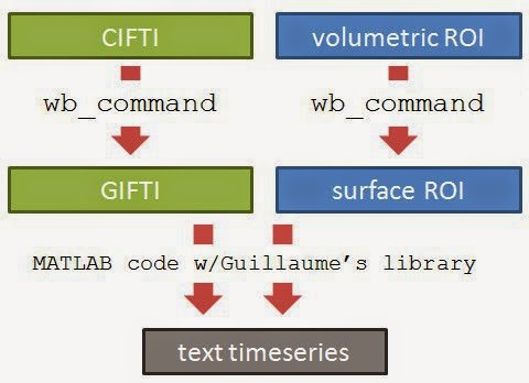
Here is an overview of the process. The logic is the simple: figure out which voxels/vertices are needed, then get the timecourses for those voxels/vertices. For HCP functional surface images there are two preliminary steps: extracting the part of the brain we want from the CIFTI file (green), and finding which vertices we want (such as by constructing a surface ROI mask, blue).

Note that it's not necessary to create a ROI to extract the timecourses; if you know which vertices you need by some other means you can read them directly in MATLAB once the GIFTI has been loaded.

unpack the CIFTI

It works best for me to think of HCP CIFTI files as archives containing the functional data for the whole brain, as a mixture of surfaces (for the cortical sheet) and volumes (for sub-cortical structures). Before reading the functional data we need to unpack the CIFTI, making GIFTI or NIfTI files, as appropriate for the part of the brain we want; the wb_command -cifti-separate program does this "unpacking" (see this post for notes about downloading HCP data, and this one about working with the Workbench wb_command command-line program). For example, if we want the functional time courses for a ROI on the left hemisphere surface, we run this at the command line:

wb_command -cifti-separate in.dtseries.nii COLUMN -metric CORTEX_LEFT out.func.gii 

where in.dtseries.nii is the path and filename of an HCP tfMRI CIFTI file (e.g. tfMRI_MOTOR_LR_Atlas.dtseries.nii), and out.func.gii is the path and filename of the GIFTI we want the program to create. The command's help has more options and explanation; in brief CORTEX_LEFT  indicates which anatomical structure to unpack, COLUMN gets timecourses, and -metric is because CORTEX_LEFT  is stored as a surface.

identify the desired vertices

There is not a one-to-one correspondence between volumetric voxels and surface vertices in the HCP functional datasets, nor a way (that I could find) to translate between the two coordinate schemes (if you know differently, please let me know!)(see update below). As a work-around, I used wb_command -volume-to-surface-mapping to translate a volumetric ROI to a surface ROI, in the same way as before:

wb_command -volume-to-surface-mapping roi.nii.gz atlas.surf.gii roi.func.gii -enclosing

where roi.nii.gz is the volumetric ROI mask, atlas.surf.gii is an atlas surface for the hemisphere containing the ROI, and roi.func.gii is the GIFTI metric file that will be created. This only works if the surface atlas, volumetric ROI, and functional CIFTI are all aligned to the same space. For the HCP data, the MNINonLinear images for each person are aligned to the MNI atlas, specifically matching the conte69 32k atlas. Thus, I made the volumetric ROI on an MNI template brain, then used Conte69.L.midthickness.32k_fs_LR.surf.gii for the atlas.surf.gii in the -volume-to-surface-mapping call. So long as the headers are correct in roi.nii.gz (i.e. the voxel size, origin, etc are correct) the ROI should be in the correct place in roi.func.gii, but view it in Workbench to be sure.

extract the vertex timecourses

Finally, we can read both the ROI and functional data GIFTI files into MATLAB, reading the vertex indices from the ROI then saving the timecourses as text:

addpath 'C:/Program Files/MATLAB/gifti-1.4';   % path to GIFTI library
roi = gifti(['d:/temp/roi.func.gii']);   % load the ROI GIFTI
inds = find(roi.cdata > 0);    % find is like which: get the vertex indices
wm = gifti([inpath 'out.func.gii']);  % load the functional GIFTI
tmp = wm.cdata(inds,:);    % get those indices' timcourses
csvwrite(['d:/temp/out.csv'], tmp);   % write as a csv text file

Now, out.csv has one column for each timepoint and one row for each vertex in the ROI.

confirming the match

We can check that the values match by opening out.func.gii in both Workbench and MATLAB:

In the image I clicked on vertex 5336 in Workbench (red arrow), which is the vertex at position 5337 in the MATLAB .cdata array (purple arrow), since MATLAB is one-based but Workbench is zero-based. The first two values of the data series shown in the Workbench Information window (red underline) match those shown in MATLAB (purple underline).

Note: I could only get Workbench to show the first two values of the timeseries if I set the little blue-arrowed button to 2; otherwise it would display only the first value. Clicking through the little blue-arrow box changes the display to different timepoints, but doesn't change the Information window that I could tell (I'm using Workbench 0.85). Note also that the "charting" interface has changed from my previous post; now you need to go through the "Chart" radio button on the upper left of the View window (right under the first tab name on my screen); I couldn't get it to write out the full timeseries in Workbench itself.


UPDATE (20 May 2014): Tim Coalson suggested that by convention the output files should be named roi.func.gii and out.func.gii, not roi.shape.gii and out.dtseries.gii as I originally wrote; I changed the commands accordingly. Tim also pointed me to the program wb_command -surface-closest-vertex, which will return the closest vertex to an arbitrary 3d coordinate. He suggests that to go the other way (from a vertex in a .surf.gii to 3d coordinates) you "could look at the coordinate of a particular vertex, and back-convert through the nifti sform to get the real-valued voxel "indices" it resides at (real-valued because it could be a third of a voxel to the right of a voxel center, etc)."