HCP: extracting timecourses from the surface files

UPDATE (29 May 2017): The new wb_command -cifti-convert -to-text function can drastically streamline this process in some cases, see this post.

----

In a previous post about viewing functional data from the Human Connectome Project (HCP) I described downloading the images then viewing them with the Connectome Workbench. This post describes a way to extract the timecourses for specific surface vertices using code, rather than one-at-a-time in the Workbench.

First, working with surfaces means working with GIFTI and CIFTI files. Many developers are creating functions that can read these files, but software is less mature and harder to find than for reading NIfTI files (MATLAB, FSL and NiBabel seem furthest along; I couldn't find one for R). The GIFTI library for MATLAB worked great ... except with HCP-derived files.Guillaume Flandin very kindly (and quickly!) changed his code to work with HCP files, making it ignore the spec-inconsistent part of those headers. By the time you read this, the files might be fixed, but for now (19 May 2014), if the GIFTI library for MATLAB gives you errors with HCP files (but not others), ask Guillaume for a copy of make sure you have version 1.4 (or newer) of the @gifti library.


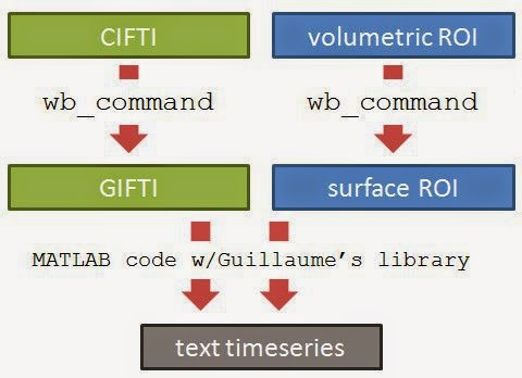
Here is an overview of the process. The logic is the simple: figure out which voxels/vertices are needed, then get the timecourses for those voxels/vertices. For HCP functional surface images there are two preliminary steps: extracting the part of the brain we want from the CIFTI file (green), and finding which vertices we want (such as by constructing a surface ROI mask, blue).

Note that it's not necessary to create a ROI to extract the timecourses; if you know which vertices you need by some other means you can read them directly in MATLAB once the GIFTI has been loaded.

unpack the CIFTI

It works best for me to think of HCP CIFTI files as archives containing the functional data for the whole brain, as a mixture of surfaces (for the cortical sheet) and volumes (for sub-cortical structures). Before reading the functional data we need to unpack the CIFTI, making GIFTI or NIfTI files, as appropriate for the part of the brain we want; the wb_command -cifti-separate program does this "unpacking" (see this post for notes about downloading HCP data, and this one about working with the Workbench wb_command command-line program). For example, if we want the functional time courses for a ROI on the left hemisphere surface, we run this at the command line:

wb_command -cifti-separate in.dtseries.nii COLUMN -metric CORTEX_LEFT out.func.gii 

where in.dtseries.nii is the path and filename of an HCP tfMRI CIFTI file (e.g. tfMRI_MOTOR_LR_Atlas.dtseries.nii), and out.func.gii is the path and filename of the GIFTI we want the program to create. The command's help has more options and explanation; in brief CORTEX_LEFT  indicates which anatomical structure to unpack, COLUMN gets timecourses, and -metric is because CORTEX_LEFT  is stored as a surface.

identify the desired vertices

There is not a one-to-one correspondence between volumetric voxels and surface vertices in the HCP functional datasets, nor a way (that I could find) to translate between the two coordinate schemes (if you know differently, please let me know!)(see update below). As a work-around, I used wb_command -volume-to-surface-mapping to translate a volumetric ROI to a surface ROI, in the same way as before:

wb_command -volume-to-surface-mapping roi.nii.gz atlas.surf.gii roi.func.gii -enclosing

where roi.nii.gz is the volumetric ROI mask, atlas.surf.gii is an atlas surface for the hemisphere containing the ROI, and roi.func.gii is the GIFTI metric file that will be created. This only works if the surface atlas, volumetric ROI, and functional CIFTI are all aligned to the same space. For the HCP data, the MNINonLinear images for each person are aligned to the MNI atlas, specifically matching the conte69 32k atlas. Thus, I made the volumetric ROI on an MNI template brain, then used Conte69.L.midthickness.32k_fs_LR.surf.gii for the atlas.surf.gii in the -volume-to-surface-mapping call. So long as the headers are correct in roi.nii.gz (i.e. the voxel size, origin, etc are correct) the ROI should be in the correct place in roi.func.gii, but view it in Workbench to be sure.

extract the vertex timecourses

Finally, we can read both the ROI and functional data GIFTI files into MATLAB, reading the vertex indices from the ROI then saving the timecourses as text:

addpath 'C:/Program Files/MATLAB/gifti-1.4';   % path to GIFTI library
roi = gifti(['d:/temp/roi.func.gii']);   % load the ROI GIFTI
inds = find(roi.cdata > 0);    % find is like which: get the vertex indices
wm = gifti([inpath 'out.func.gii']);  % load the functional GIFTI
tmp = wm.cdata(inds,:);    % get those indices' timcourses
csvwrite(['d:/temp/out.csv'], tmp);   % write as a csv text file

Now, out.csv has one column for each timepoint and one row for each vertex in the ROI.

confirming the match

We can check that the values match by opening out.func.gii in both Workbench and MATLAB:

In the image I clicked on vertex 5336 in Workbench (red arrow), which is the vertex at position 5337 in the MATLAB .cdata array (purple arrow), since MATLAB is one-based but Workbench is zero-based. The first two values of the data series shown in the Workbench Information window (red underline) match those shown in MATLAB (purple underline).

Note: I could only get Workbench to show the first two values of the timeseries if I set the little blue-arrowed button to 2; otherwise it would display only the first value. Clicking through the little blue-arrow box changes the display to different timepoints, but doesn't change the Information window that I could tell (I'm using Workbench 0.85). Note also that the "charting" interface has changed from my previous post; now you need to go through the "Chart" radio button on the upper left of the View window (right under the first tab name on my screen); I couldn't get it to write out the full timeseries in Workbench itself.


UPDATE (20 May 2014): Tim Coalson suggested that by convention the output files should be named roi.func.gii and out.func.gii, not roi.shape.gii and out.dtseries.gii as I originally wrote; I changed the commands accordingly. Tim also pointed me to the program wb_command -surface-closest-vertex, which will return the closest vertex to an arbitrary 3d coordinate. He suggests that to go the other way (from a vertex in a .surf.gii to 3d coordinates) you "could look at the coordinate of a particular vertex, and back-convert through the nifti sform to get the real-valued voxel "indices" it resides at (real-valued because it could be a third of a voxel to the right of a voxel center, etc)."

clever RSA: "Hippocampal Activity Patterns Carry Information about Objects in Temporal Context"

There's an interesting use of RSA (representational similarity analysis) in a recent paper by Hsieh et al. This bit of Figure 1 summarizes the dataset: in each scanning run people were shown the same set of object images, each image shown for 1 sec, followed by a 5 sec inter-stimulus interval. The people pushed a button to answer a semantic question about each image (e.g. "Is the presented object living?"), with a different semantic question each run. A key part of the experimental design is the sequences in which the objects were presented.

The images made up six sequences, which were learned right before scanning, then shown three times in each of the five scanning runs. As shown here, different objects were used in the Fixed, X, Y, and Random sequences; two objects were shared between the X sequences, and three between the Y sequences. Each sequence had the images shown in the order in the figure, except for the Random sequence, which was randomly different each time (the camel could be first one time, then third the next).

This set of sequences made it possible to look for order and identity effects: once you saw the rake, you would know (since the participants memorized the sequences before scanning) that you would see the truck next, followed by the cabinet, etc. If you saw the rhino you would know the drill and strawberry would be next, but not whether the chair or elk would be in the fourth position. Seeing the camel first would have you expect the tractor, shears, stand, or pineapple to be next, but not which one (though by the fourth object you'd know which of the Random set hadn't yet been shown).

The presented results are all ROI-based, with the hippocampus, parahippocampal cortex (PHc), and perirhinal cortex (PRc). The ROIs were individually drawn for each person,  but I didn't see a list of how many voxels went into the ROIs for each person, or a mention of how much variability there was in the size across people and ROIs. If they kept the voxels at the acquired 3.2×3.2×3.0 mm, I'd guess there'd be less than 20 voxels in each ROI, but it would be nice to have had the exact counts. (And I wonder if they looked outside the ROIs; seems likely, since they acquired whole-brain images.)

Anyway, they created parameter estimate images (fit a canonical HRF) for each image presentation (90 per run), then created an RSA matrix (with Pearson correlation) for each same-sequence repetition within a run, then averaged those three matrices to get one matrix per sequence per run, then averaged across runs, then across people (Figure 3).

I'm not going to mention everything they presented, just the analysis summarized in Figure 4, which is copied in part here. The left pane shows the RSA matrix when everything except the Random sequence goes into the average: nice dark red colors (high correlation) along the diagonal, dropping off moving away from the diagonal (note the weird matlab-default color scheme: yellow, green, and cyan are near zero).

The clever bit is how they made the RSA matrices for the Random sequences: based on position or object (Figure 3). For position, they did the RSA with the true sequences: correlating the first-presented image against the first, even though they were different images. There's very little correlation in the upper left corner of this matrix, but more in the lower right - perhaps because the last few images could be guessed. Then, they did the RSA based on object: correlating the same images together (camel to camel), regardless of order. They used these three RSA matrices to test their hypotheses (Figure 8): which ROIs had information about object identity? Which about the order? Which had both?

One last comment: Figure 5 makes me wish for more supplemental information ... these are very strong correlations for the noisiness of the data (and the small size of the correlations making up the "similarity change" metric). It would have been nice to see error bars on these points, or something like the range across the five runs for each person. The individual graphs ("same obj+pos" and "same obj") separately, rather than just the difference, would also be interesting, and perhaps explain why some people have a negative similarity change.


Hsieh, L., Gruber, M., Jenkins, L., & Ranganath, C. (2014). Hippocampal Activity Patterns Carry Information about Objects in Temporal Context Neuron, 81 (5), 1165-1178 DOI: 10.1016/j.neuron.2014.01.015