balanced accuracy: what and why?

I was a bit thrown at OHBM by mentions of using "balanced" accuracy to describe classification performance ... what's wrong with "regular" accuracy? Well, nothing is wrong with "regular" accuracy, if your dataset is already balanced (meaning equal numbers of trials in each class and cross-validation fold, which I very highly recommend). But if your test set is not balanced, "balanced" accuracy is probably better than "regular".

At left is an example of a confusion matrix produced by a classifier, where the test set was balanced, with 10 examples of class face, and 10 of class place. The classifier did quite well: 9 of the 10 face examples were (correctly) labeled face, and 8 of the 10 place examples were (correctly) labeled place. For lack of a better term, what I'll call "regular" or "overall" accuracy is calculated as shown at left: the proportion of examples correctly classified, counting all four cells in the confusion matrix. Balanced accuracy is calculated as the average of the proportion corrects of each class individually. In this example, both the overall and balanced calculations produce the same accuracy (0.85), as will always happen when the test set has the same number of examples in each class.

This second example is the same as the first, but I took out one of the place test examples: now the testing dataset was not balanced, as it has 10 face examples, but only 9 place examples. As you can see, now the overall accuracy is a bit higher than the balanced.


It's easy to generate more confusion matrices to get a feel for how the two ways of calculating accuracy differ, such as with this R code:

 c.matrix <- rbind(c(1,0),   
                   c(1,1));  
 sum(diag(c.matrix))/sum(c.matrix);  # "overall" proportion correct  
 first.row <- c.matrix[1,1] / (c.matrix[1,1] + c.matrix[1,2])  
 second.row <- c.matrix[2,2] / (c.matrix[2,1] + c.matrix[2,2])  
 (first.row + second.row)/2; # "balanced" proportion correct  

So, should we use balanced accuracy instead of overall? Yes, it's probably better to use balanced accuracy when there's just one test set, and it isn't balanced. I tend to be extremely skeptical about interpreting classification results when the training set is not balanced, and would want to investigate a lot more before deciding that balanced accuracy reliably compensates for unbalanced training sets. However, it's probably fine to use balanced accuracy with unbalanced test sets in situations like cross-classification, where a classifier is trained once on a balanced training set (e.g., one person's dataset), and then tested once (e.g., another person's dataset). Datasets requiring cross-validation need to be fully balanced, because the each testing set contributes to the training set in other folds.

For more, see Brodersen, Kay H., Cheng Soon Ong, Klaas E. Stephan, and Joachim M. Buhmann. 2010. "The balanced accuracy and its posterior distribution." DOI: 10.1109/ICPR.2010.764

"Assessment of tonotopically organised subdivisions in human auditory cortex using volumetric and surface-based cortical alignments"

Given my occasional forays into surface analysis (and lack of conviction that it's necessarily a good idea for fMRI), I was intrigued by some of the analyses in a recent paper from Dave Langers ("Assessment of tonotopically organised subdivisions in human auditory cortex using volumetric and surface-based cortical alignments").

For task fMRI, the most transparent way to compare different analysis methods seems to use a task that's fairly well defined and anatomically predictable. Motion and primary senses are probably most tractable; for example a task that has blocks of finger-tapping and toe-wiggling should produce very strong signal, and be distinguishable in motor cortex. This gives a basis of comparison: with which method do we see the finger and toe signals most distinctly?

Langers (2014) investigated tonotopic maps in auditory cortex, which map the frequency of heard sounds, using volumetric and surface analysis. While tonotopic maps are not fully understood (see the paper for details!), this is a well-defined question for comparing surface and volumetric analysis of fMRI data: we know where the primary auditory cortex is located, and we know when people were listening to which sounds. He used a Hotelling's T2-related statistic for describing the "tonotopic gradient vectors" which reminds me a bit of cvMANOVA and the LD-t, but I'll just concentrate on the surface vs. volume aspects here.

This is Figure 2 from the paper, which, gives a flowchart of the procedures for the surface and volume versions of the analysis. He mapped the final volumetric results onto a (group) surface to make it easier to compare the surface and volume results, but the preprocessing and statistics were carried out separately (and it seems to me, reasonably): SPM8 for volumetric, freesurfer for surface. The fMRI voxels were small - just 1.5 x 1.5 . 1.5 mm, which is plausible to support surface analysis.

So, which did better, surface or volume? Well, to quote from the Discussion, "... the activation detected by the surface-based method was stronger than that according to the volumetric method. At the same time, the related statistical confidence levels were more or less the same." The image below is part of Figure 4 from the paper, showing a few of the group-level results (take a look at the full paper). As he observes, "The surface-based results had a noisier appearance than the volumetric ones, in particular for the frequency-related outcomes shown in Figure 4c–e."

So, in this paper, while the surface analysis seemed to result in better anatomic alignments between people, the activation maps were not clearer or more significant. I'd very much like to see more comparisons of this type (particularly with HCP processing, given its unique aspects), to see if this is a common pattern, or something unique to tonotopic maps in auditory cortex and this particular protocol.


Langers, D. (2014). Assessment of tonotopically organised subdivisions in human auditory cortex using volumetric and surface-based cortical alignments Human Brain Mapping, 35 (4), 1544-1561 DOI: 10.1002/hbm.22272

positive control analyses and checking data quality

I've long advocated that much pain can be avoided if analysis of a new dataset is begun with positive control analyses: classifying (or whatever) something that should produce a very strong signal in easy-to-identify regions. Button-presses often are good controls (particularly if the button boxes were in different hands): when classifying whether the left-hand or right-hand was moved (totally ignoring the experimental conditions), do you find motor areas? Classifying the presence or absence of visual stimuli is also a good, strong control. Once a positive control is found, some of the analysis choices and data quality checks can be run on the control analysis then carried over to the target analysis, reducing the chance of exploiting too many experimenter degrees of freedom.

Another reason to start with positive control analyses is simply to identify problems in the dataset. If the control analysis fails in a particular person, why? Were the event timings mislabeled? Movement too high? Preprocessing failed? I'd be very worried about interpreting the results of a subtle cognitive task in a person whose data is of too poor a quality to support classifying something as strong as hand movements.

The rest of this post is an example of what positive control analyses can look like, and how their results compare to measures of general dataset quality. Several practiCal fMRI posts were very useful for thinking about how to visualize the image quality, particularly this one describing temporal SNR and this one showing examples of high-quality images.

average the fMRI timeseries for each voxel

First, run-wise mean images. These are simply the average of the functional timeseries for each voxel, each run and person separately. I calculated these on the images after preprocessing, but before voxelwise normalization. This is evaluating the quality of the images as they "arrive" for MVPA; in this case, after motion-correction, slice-time correction, and spatial normalization to an anatomic template. We thus expect the slices to look fairly similar in all people (because of the normalization), basically like fuzzy anatomical images.

The images below show two slices (one coronal, one axial) of the mean fMRI image for four runs in six people from two datasets (people in rows, runs in columns). The first image shows a dataset with fairly decent spatial normalization, the second, not-so-good spatial normalization (the images should enlarge if clicked).

A dataset with fairly decent spatial normalization. While the images vary a bit (e.g., subject 17 is rather "pointy" compared to the others), they are all orientated correctly and capture the same brain structures.

A dataset with not-so-good spatial normalization. Note that each person is pretty consistently normalized with themselves (i.e., the images in the four runs within each person are similar), but vary quite a bit between people. For example, sub7's brain looks "short", and when viewed in 3d, is clearly tilted.

In my estimation, analysis should not proceed on this dataset: spatial normalization needs to be improved, or analysis should be performed in subject (native) space.

standard deviation of the fMRI timeseries for each voxel

As described by practiCal fMRI, images of the standard deviation of the fMRI timeseries are useful for spotting motion or other artifacts; see his post for more details. Basically, dimmer is better for these images, and we want to be able to see some brain structure. As with the mean images, these are simply calculating the standard deviation of each voxel's timeseries, separately within each run, using the post-preprocessing functional images. All image voxels were included, not just those in the brain mask, to allow spotting of blurry edges and ghosts.

The top part of this image are the standard deviations. This follows the convention of the mean images: subjects in the rows, four runs in the columns, with coronal slices first, then axial slices, both of the same 3d image. All images have the same color scaling, so brightness can be compared between runs and people.

Subject 34 is the best of these three people: the images for the four runs are pretty equally dark, but the brain outline and structure are visible. Subject 37 has the second and first runs much brighter and blurrier than the third and fourth runs; the first run in subject 36 is also brighter and blurrier than the others. These runs had more movement artifacts, reflected here as higher standard deviation.

The bottom part of this image is the accuracy from a positive control searchlight analysis in these same three people. In this case, the control analysis was classifying whether a particular image was from a cue or target/response trial segment, and we expect visual and motor areas to classify. (If you're curious, it was leave-one-run-out cross-validation within each person, linear SVM, c=1, 3-voxel radius searchlights, two balanced classes.) The overlay is color-scaled to show voxels with accuracy of 0.6 as red, 1 (perfect) as brightest yellow, not showing voxels with accuracy less than 0.6 (chance = 0.5). (I used knitr to make all the images in this post; see this demo for similar code.)

The accuracies and standard deviation are consistent in these images: sub34 has the lowest standard deviation (and highest temporal SNR, though this isn't shown here) and highest classification accuracy; sub36 and sub37 have fewer high-classifying searchlights. The relationship between image quality in these diagnostic tests and control classification accuracy is not always this clear, but I have seen it pretty often, and it should exist; by definition, the control classification should succeed in people with decent image quality. If it does not, the dataset should be checked for errors, such as mislabeled event timing files.

There's no magic threshold for image quality, nor perfect strategy for recovering signal from high-movement runs. But I would be very hesitant to continue analyzing a person without clear signal in the control analysis, particularly if they stand out in the mean and standard deviation images.

How to do cross-validation? Have to partition on the runs?

People sometimes ask why many MVPA studies use leave-one-run-out cross-validation (partitioning on the runs), and if it's valid to set up the cross-validation in other ways, such as leaving out individual trials. Short answer: partitioning on the runs is a sensible default for single-subject analyses, but (as usual with fMRI) other methods are also valid in certain situations.

As I've written before, cross-validation is not a statistical test itself, but rather the technique by which we get the statistic we want to test (see this for a bit more on doing statistical testing). My default example statistic is accuracy from a linear SVM, but these issues apply to other statistics and algorithms as well.

Why is partitioning on the runs a sensible default? A big reason is that scanner runs (also called "sessions") are natural breaks in fMRI datasets: a run is the period in which the scanner starts, takes a bunch of images at intervals of one TR, then stops. Images from within a single scanner run are intrinsically more related to each other than to images from different runs, partly because they were collected closer together in time (so the subject's mental state and physical position should be more similar; single hemodynamic responses can last more than one TR), and because many software packages perform some corrections on each run individually (e.g., SPM motion correction usually aligns each volume to the first image within its run). The fundamental nature of temporal dependency is reflected in the terminology of many analysis programs, such as "chunks" in pyMVPA and "bricks" in afni.

So, since the fMRI data within each person is structured into runs, it makes sense to partition on the runs. It's not necessary to leave-one-run-out, but if you're not leaving some multiple number of runs out for the cross-validation, you should verify that your (not run-based) scheme is ok (more later). By "some multiple number of runs" I mean leaving out two, three, or more runs on each cross-validation fold. For example, if your dataset has 20 short runs you will likely have more stable (and significant) performance if you leave out two or four runs each fold rather than just one (e.g., Permutation Tests for Classification. AI Memo 2003-019). Another common reason to partition with multiple runs is if you're doing some sort of cross-classification, like training on all examples from one scanning day and testing on all examples from another scanning day. With cross-classification there might not be full cross-validation, such as if training on "novel" runs and testing on "practiced" runs is of interest for an experiment, but training on "practiced" runs and testing with "novel" runs is not. There's no problem with these cross-classification schemes, so long as one set of runs is used for training, and another (non-intersecting) set of runs for testing in an experiment-sensible (and ideally a priori) manner.

But it can sometimes be fine to do cross-validation with smaller bits of the dataset than the run, such as leaving out individual trials or blocks. The underlying criteria is the same, though: are there sensible reasons to think that the units you want to use for cross-validation are fairly independent? If your events are separated by less than 10 seconds or so (i.e., HRF duration) it's hard to argue that it'd be ok to put one event in the training set and the event after it into the testing set, since there will be so much "smearing" of information from the first event into the second (and doubly so if the event ordering is not perfectly balanced). But if your events are fairly well-spaced (e.g. a block design with 10 second action blocks separated by 20 seconds of rest), then yes, cross-validating on the blocks might be sensible, particularly if preprocessing is aimed at isolating the signal from individual blocks.

If you think that partitioning on trials or blocks, rather than full runs, is appropriate for your particular dataset and analysis, I suggest you include an explanation of why you think it's ok (e.g., because of the event timing), as well as a demonstration that your partitioning scheme did not positively bias the results. What demonstration is convincing necessarily varies with dataset and hypotheses, but could include "random runs" and control analyses. I described "random runs" in The impact of certain methodological choices ... (2011); the basic idea is to cross-validate on the runs, but then randomly assign the trials to new "runs", and do the analysis again (i.e., so that trials from the same run are mixed into the training and testing sets). If partitioning on the random runs and the real runs produce similar results, then mixing the trials didn't artificially increase performance, and so partitioning other than on the runs (like leaving out individual blocks) is probably ok. Control analyses are classifications that shouldn't work, such as using visual cortex to classify an auditory stimulus. If such negative control analyses aren't negative (can classify) in a particular cross-validation scheme, then that cross-validation scheme shouldn't be trusted (the training and testing sets are not independent, or some other error is occurring). But if the target analysis (e.g., classifying the auditory stimuli with auditory cortex) is successful while the control analysis (e.g., classifying the auditory stimuli with visual cortex) is not, and both use the same cross-validation scheme, then the partitioning was probably ok.

This post has focused on cross-validation when each person is analyzed separately. However, for completeness, I want to mention that another sensible way to partition fMRI data is on the people, such as with leave-one-subject-out cross-validation. Subjects are generally independent (and so suitable "chunks" for cross-validation), unless the design includes an unusual population (e.g., identical twins) or design (e.g., social interactions).

a nice "Primer on Pattern-Based Approaches to fMRI"

John-Dylan Haynes has a new MVPA review article out in Neuron, "A Primer on Pattern-Based Approaches to fMRI" (full citation below). I say "new" because he (and Rees) was the author of one of the first MVPA overview articles ("Decoding mental states from brain activity in humans"), back in 2006. As with the earlier article, this is a good introduction to some of the main methods and issues; I'll highlight a few things here, in no particular order.

At left is part of Figure 4, which nicely illustrates four different "temporal selection" options for event-related designs. The red and green indicate the two different classes of stimuli (cats and dogs), with the black line the fMRI signal in a single voxel across time.

I often refer to these as "temporal compression" options, but like "temporal selection" even better: we are "selecting" how to represent the temporal aspect of the data, and "compression" isn't necessarily involved.

John-Dylan Haynes (quite properly, in my opinion) recommends permutation tests (over binomial and t-tests) for estimating significance, noting that one of their (many) benefits is in detecting biases or errors in the analysis procedure.

Overall, I agree with his discussion of spatial selection methods (Figure 3 is a nice summary), and was intrigued by the mention of wavelet pyramids as a form of spatial filtering. I like the idea of spatial filtering to quantify the spatial scale at which information is present, but haven't run across a straightforward implementation (other than searchlight analysis); wavelet pyramids might need more investigation.

I also appreciate his caution against trying too many different classifiers and analysis procedures on the same dataset, pointing out that this can cause "circularity and overfitting". This problem is also sometimes referred to as having too many experimenter degrees of freedom: if you try enough versions of an analysis you can probably find one that's "significant." His advice to use nested cross-validation strategies (e.g., tuning the analysis parameters on a subset of the subjects) is solid, if sometimes difficult in practice because of the limited number of available subjects. The advice to use an analysis that "substantially decreases the number of free parameters" is also solid, if somewhat unsatisfying: I often advise people to use linear SVM, c=1 as the default analysis. While tuning parameters and testing other classifiers could conceivably lead to a higher accuracy, the risk of false positives from exploiting experimenter degrees of freedom is very real.

I also like his inclusion of RSA and encoding methods in this "primer". Too often we think of classifier-based MVPA, RSA, and encoding methods as unrelated techniques, but it's probably more accurate to think of them as "cousins," or falling along a continuum.

It's clear by now that I generally agree with his issue framing and discussion, though I do have a few minor quibbles, such as his description of MVPA methods as aimed at directly studying "the link between mental representations and corresponding multivoxel fMRI activity patterns". I'd assert that MVPA are also useful as a proxy for regional information content, even without explicit investigation of cognitive encoding patterns. But these are minor differences; I encourage you to take a look at this solid review article.


  Haynes JD (2015). A Primer on Pattern-Based Approaches to fMRI: Principles, Pitfalls, and Perspectives. Neuron, 87 (2), 257-70 PMID: 26182413

demo: permutation tests for within-subjects cross-validation

This R code demonstrates how to carry out a permutation test at the group level, when using within-subjects cross-validation. I describe permutation schemes in a pair of PRNI conference papers; see DOI:10.1109/PRNI.2013.44 for an introduction and single subjects, and this one for the group level, including the fully balanced within-subjects approach used in the demo. A blog post from a few years ago also describes some of the issues, using examples structured quite similarly to this demo.

For this demo I used part of the dataset from doi:10.1093/cercor/bhu327, which can be downloaded from the OSF site. I did a lot of temporal compression with this dataset, which is useful for the demo, since only about 18 MB of files need to be downloaded.Unfortunately, none of the analyses we did for the paper are quite suitable to demonstrate simple permutation testing with within-subjects cross-validation, so this demo performs a new analysis. The demo analysis is valid, just not really sensible for the paper's hypotheses (so, don't be confused when you can't find it in the paper!).

The above figure is generated by the demo code, and shows the results of the test. The demo uses 18 subjects' data, and their null distributions are shown as blue histograms. The true-labeled accuracy for each person is plotted as a red line, and listed in the title, along with its p-value, calculated from the shown null distribution (the best-possible p-value, 1/2906, rounds to 0).

The dataset used for the demo has no missings: each of the people has six runs, with four examples (two of each class) in each run. Thus, I can use a single set of labels for the permutation test, carrying out the relabelings and classifications in each person individually (since it's within-subjects cross-validation), but with the null distribution for each person built from the same relabelings. Using the same relabelings in each person allows the group-level null distribution (green, in the image above) to be built from the across-subjects average accuracy for each relabeling. In a previous post I called this fully-balanced strategy "single corresponding stripes", illustrated with the image below; see that post (or the demo code) for more detail.

The histogram for the across-subjects means (green histogram; black column) is narrower than the individual subject's histograms. This is sensible: for any particular permutation relabeling, one person might have a high accuracy, and another person a low accuracy; averaging the values together gives a value closer to chance. Rephrased, each individual has at least one permutation with very low (0.2) accuracy (as can be seen in the blue histograms). But different labelings made that low accuracy in each person, so the lowest group-mean accuracy was 0.4.

The group mean of 0.69 was higher than all the permuted-label group means, giving a p-value of 0.0003 = 1/2906 (2906 permutation relabelings were run, all possible). The equivalent t-test is shown in the last panel, and also produces a very significant p-value.

start planning: PRNI 2016

Start planning: the 6th International Workshop on Pattern Recognition in Neuroimaging will be held at the University of Trento (Italy), (probably) 21-24 June 2016. PRNI is an OHBM satellite conference, generally held several days before and somewhat geographically near the OHBM conference, which next year is in Geneva, Switzerland, 26-30 June 2016. Once the hosting is sorted out the website will be (as for past meetings) linked from www.prni.org.

The paper deadline will be mid-March 2016, perhaps with a later deadline for short abstract-only poster submissions. Previous workshops' papers were published by IEEE; search for "Pattern Recognition in Neuroimaging". Conference papers are standard in many engineering-related fields, but might be unfamiliar for people from a psychology or neuroscience background. Basically, PRNI papers are "real" publications: they are peer-reviewed, published in proceedings, indexed, and cite-able. The paper guidelines aren't settled yet, but will likely be similar to those of previous years. MVPA methods papers (applications, statistical testing, ...) are a good fit for PRNI; not just fMRI, but any neuroimaging modality is welcome.

UPDATE 10 November 2015: prni.org now has information about PRNI 2016 (including the call for papers), and we'll be updating the website as time goes on. You can also follow on twitter @PRNI2016 or facebook.

R? python? MATLAB?

I've been asked a few times why I use R for MVPA, and what I think people just getting into MVPA should use. I don't think that there is a universally "best" package for MVPA (or neuroimaging, or statistics), but here are some musings.

The question as to why I personally started using R for MVPA is easy: I started before MVPA packages were available, so I had to write my own scripts, and I prefer scripting in R (then and now). Whether to keep using my own scripts or switch to pyMVPA (or some other package) is something I reconsider occasionally.

A very big reason to an established package is that it's a known quantity: coding bugs have hopefully been caught, and analyses can be reproduced. Some packages are more open (and have more stringent tests) than others, but in general, the more eyes that have studied the code and tried the routines, the better. This need for openness was one of my motivations for starting this blog: to post bits of code and detailed methods descriptions. I think the more code and details we share (blog, OSF, github, whatever), the better, regardless of what software we use (and I wish code was hosted by journals, but that's another issue).

I'm a very, very big fan of using R for statistical analyses, and of knitr (sweave and RMarkdown are also viable options in R) for documenting the various analyses, results, impressions, and decisions as the research progresses (see my demo here), regardless of the program that generated the raw data. My usual workflow is to switch to knitr once an analysis reaches the "what happened?" stage, regardless of the program that generated the data being analyzed (e.g., I have knitr files summarizing the motivation, procedure, and calculating results from cvMANOVA analyses run in MATLAB). Python has the iPython Notebook, which is sort of similar to knitr (I don't think as aesthetically pleasing, but that's a matter of taste); I don't think MATLAB has anything equivalent. Update 12 August 2015 (Thanks, Dov!): MATLAB comes with Publishing Markup, which (at a quick glance) looks similar to RMarkdown.

All neuroimaging (and psychology, neuroscience, ...) graduate students should expect to learn a proper statistical analysis language, by which I mostly mean R, with MATLAB and python coming in as secondary options. In practice, if you have proficiency in one of these programs you can use the others as needed (the syntax isn't that different), or have them work together (e.g., calling MATLAB routines from R; calling R functions from python). The exact same MVPA can be scripted in all three languages (e.g., read in NIfTI images, fit a linear SVM, write the results into a file), and I don't see that any one of the three languages is clearly best or worst. MATLAB has serious licensing issues (and expense); python dependencies can be a major headache, but which program is favored seems to go more with field (engineers for MATLAB, statisticians for R) and personal preference than intrinsic qualities.

So, what should a person getting started with MVPA use? I'd say an R, python, or MATLAB-based package/set of scripts, with which exact one depending on (probably most important!) what your colleagues are using, personal preference and experience (e.g, if you know python in and out, try pyMVPA), and what software you're using for image preprocessing (e.g., if SPM, try PRoNTO). Post-MVPA (and non-MVPA) investigations will likely involve R at some point (e.g., for fitting mixed models or making publication-quality graphs), since it has the most comprehensive set of functions (statisticians favor R), but that doesn't mean everything needs to be run in R.

But don't start from scratch; use existing scripts/programs/functions as much as possible. You should mostly be writing code for analysis-specific things (e.g., the cross-validation scheme, which subjects are patients, which ROIs to include), not general things (like reading NIfTI images, training a SVM, fitting a linear model). Well-validated functions exist for those more general things (e.g., oro.nifti, libsvm); use them.

Notes from the OHBM 2015 "Statistical Assessment of MVPA Results" Morning Workshop

Thanks to everyone that attended and gave feedback on the OHBM morning workshop "Statistical Assessment of MVPA Results" that Yaroslav Halchenko and I organized! We've received several requests for slides and materials related to the workshop, so I'll collect them here. It appears that material from the meeting will also be searchable from links on the main OHBM 2015 page. As always, all rights are reserved, and we expect to be fully cited, acknowledged, and consulted for any uses of this material.

I started the workshop off with a tutorial on permutation testing aimed at introducing issues particularly relevant for MVPA (and neuroimaging datasets in general). I'll eventually post a version of the slides, but some of the material is already available in more detail in two PRNI conference papers:

• Etzel, J.A. 2015. MVPA Permutation Schemes: Permutation Testing for the Group Level. 5th International Workshop on Pattern Recognition in NeuroImaging (PRNI 2015). Stanford, CA, USA. In press, full text here, and in ResearchGate.
• Etzel, J.A., Braver, T.S., 2013. MVPA Permutation Schemes: Permutation Testing in the Land of Cross-Validation. 3rd International Workshop on Pattern Recognition in NeuroImaging (PRNI 2013). IEEE, Philadelphia, PA, USA. DOI:10.1109/PRNI.2013.44. Full text here, and in ResearchGate.

Next, Johannes Stelzer gave a talk entitled "Nonparametric methods for correcting the multiple comparisons problem in classification-based fMRI", the slides for which are available here.

Then, Nikolaus Kriegeskorte gave a talk entitled "Inference on computational models from predictions of representational geometries", the slides for which are available here.

Finally, Yaroslav Halchenko finished the session with a talk giving an "Overview of statistical evaluation techniques adopted by publicly available MVPA toolboxes", the slides for which are available here. 

resampling images with wb_command -volume-affine-resample

I often need to resample images without performing other calculations, for example, making a 3x3x3 mm voxel version of an anatomical image with 1x1x1 mm voxels for use as an underlay. This can be done with ImCalc in SPM, but that's a bit annoying, as it requires firing up SPM, and only outputs two-part NIfTI images (minor annoyances, but still).

The wb_command -volume-affine-resample program gets the resampling done at the command prompt with a single long command:

 wb_command -volume-affine-resample d:/temp/inImage.nii.gz d:/temp/affine.txt d:/temp/matchImage.nii CUBIC d:/temp/outImage.nii  

If the wb_command program isn't on the path, run this at the command prompt, from wherever wb_command.exe (or the equivalent for your platform) is installed. A lot of  things need to be specified:

• inImage.nii.gz is the image you want to resample (for example, the 1x1x1 mm anatomical image)
• affine.txt is a text file with the transformation to apply (see below)
• matchImage.nii is the image with the dimensions you want the output image to have - what inImage should be transformed to match (for example, the 3x3x3 mm functional image)
• CUBIC is how to do the resampling; other options are TRILINEAR and ENCLOSING_VOXEL
• outImage.nii is the new image that will be written: inImage resampled to match matchImage; specifying a outImage.nii.gz will cause a gzipped NIfTI to be written.

The program writes outImage as a one-file (not a header-image pair) NIfTI. It takes input images as both compressed (i.e., .nii.gz) and uncompressed (i.e., .nii) one-file NIfTIs, but didn't like a header-image pair for input.

You need to specify an affine transform, but I don't want to warp anything so the matrix is all 1s and 0s; just put this matrix into a plain text file (I called it affine.txt):

 1 0 0 0  
 0 1 0 0  
 0 0 1 0  

UPDATE 24 May 2016: similar demo using afni 3dresample.
UPDATE 20 May 2015: Changed the resampling method to CUBIC and added a note that the program can output compressed images, as suggested by Tim Coalson.

MVPA on the surface: to interpolate or not to interpolate?

A few weeks ago I posted about a set of ROI-based MVPA results using HCP images, comparing the results of doing the analysis with the surface or volume version of the dataset. As mentioned there, there hasn't been a huge amount of MVPA with surface data, but there has been some, particularly using the algorithms in Surfing (they're also in pyMVPA and CoSMoMVPA), described by Nikolaas Oosterhof (et al., 2011).

The general strategy in all MVPA (volume or surface) is usually to minimize changing the fMRI timeseries as much as possible; motion correction is pretty much always unavoidable, but is sometimes the only whole-brain image manipulation applied: voxels are kept in the acquired resolution, not smoothed, not slice-time corrected, not spatially normalized to an atlas (i.e., each individual analyzed in their own space, allowing the people to have differently-shaped brains). The hope is that this minimal preprocessing will maximize spatial resolution: since we want to detect voxel-level patterns, let's change the voxels as little as possible.

The surface searchlighting procedure in Surfing follows this minimum-voxel-manipulation strategy, using a combination of surface and volume representations: voxel timecourses are used, but adjacency determined from the surface representation. Rephrased, even though the searchlights are drawn following the surface (using a high-resolution surface representation), the functional data is not interpolated, but rather kept as voxels: each surface vertex is spatially mapped to a voxel, allowing multiple vertices to fall within a single voxel in highly folded areas. Figure 2 from the Surfing documentation  shows this dual surface-and-volume way of working with the data, and describes the voxel selection procedure in more detail. In the way I've described my own searchlight code, the Surfing procedure results in a lookup table (which voxels constitute the searchlight for each voxel) where the searchlights are shaped to follow the surface in a particular way.

It should be possible to do this (Surfing-style, surface searchlights with voxel timecourses) with the released HCP data. The HCP volumetric task-fMRI images are spatially normalized to the MNI atlas, which will simplify things, since the same lookup table can be used with all people, though possibly at the cost of some spatial normalization-caused distortions. [EDIT 17 May 2015: Nick Oosterhof pointed out that even with MNI-normalized volumetric fMRI data, the subject-space surfaces could be used to map adjacent vertices, in which case each person would need their own lookup table. With this mapping, the same i,j,k-coordinate voxel could have different searchlights in different people.]

The HCP task fMRI data is also available as (CIFTI-format) surfaces, which were generated by resampling the (spatially-normalized) voxels' timecourses into surface vertices. The timecourses in the HCP surface fMRI data have thus been interpolated several times, including to volumetric MNI space and to the vertices.

Is this extra interpolation beneficial or not? Comparisons are needed, and I'd love to hear about any if you've tried them. The ones I've done so far are with comparatively large parcels, not searchlights, and certainly not the last word.

grey matter musings

fMRI data is always acquired as volumes,  usually (in humans) with voxels something like 2x2x2 to 4x4x4 mm in size. Some people have argued that for maximum power analyses should concentrate on the grey matter, ideally as surface representations. This strikes me as a bit dicey: fMRI data is acquired at the same resolution all over the brain; it isn't more precise where the brain is more folded (areas with more folding have closer-spaced vertices in the surface representation, so multiple vertices can fall within a single voxel).

But how much of a problem is this? How does the typically-acquired fMRI voxel size compare to the size of the grey matter? Trying to separate out fMRI signals from the grey matter is a very different proposition if something like ten voxels typically fit within the ribbon vs. just one.

Fischl and Dale (2000, PNAS, "Measuring the thickness of the human cerebral cortex from magnetic resonance images") answers my basic question of how wide the grey matter typically is in adults: 2.5 mm. This figure (Figure 3) shows the histogram of grey matter thickness that they found in one person's cortex; in that person, "More than 99% of the surface is between 1- and 4.5-mm thick."

So, it's more typical that the grey matter is one fMRI voxel wide than multiple.  A 4x4x4 mm functional voxel will be wider than nearly all grey matter; most voxels within the grey matter will contain some fractional proportion, not just grey matter. Things are better with 2x2x2 mm acquired voxels, but it will still be the case that a voxel falling completely into the grey matter will be fairly unusual, and even these totally-grey voxels will surrounded on several sides by non-grey matter voxels. To make it concrete, here's a sketch of common fMRI voxel sizes on a perfectly straight grey matter ribbon.

This nearness of all-grey, some-grey, and no-grey voxels is problematic for analysis. An obvious issue is blurring from motion: head motion of a mm or two within a run is almost impossible to avoid, and will totally change the proportion of grey matter within a given voxel. Even if there was no motion at all, the different proportions of grey matter causes problems ("partial volume effects"; see for example): if all the signal came from the grey matter, the furthest-right 2 mm voxels in the image above would be less informative than the adjacent 2 mm voxel which is centered in the grey, just because of the differing proportion grey. Field inhomogeneity effects, scanner drift, slice-time correction, resampling, smoothing, spatial normalization, etc. cause further blurring.

But the cortex grey matter is of course not perfectly flat like in the sketch: it's twisted and folded in three dimensions, like shown here in Figure 1 from Fischl and Dale (2000). This folding leads complicates things further: individual voxels still have varying amounts of grey matter, but can also encompass structures far apart if measured along the surface.





This figure is panels C (left) and D (right) from Figure 2 of Kang et al. (2007, Magnetic Resonance Imaging. Improving the resolution of functional brain imaging), and illustrates some of the "complications". The yellow outline at left is the grey-white boundary on an anatomical image (1x1x1 mm), with two functional voxels superimposed, one in red and one in green (the squares mark the voxels' corners; they had 1.88x1.88x5 mm functional voxels). The right pane shows the same two voxels' locations in a surface flat map (dark areas grey matter, light areas white). In their words, "Although the centers of the filled squares in the corners of the red and green functional voxels in (C) are the same distance apart in the 3-D space and points in the same voxel must be within 5.35 mm, functional activations in the red voxel spread to areas over 30 mm apart on the flat map, while activations in the green voxel remain close to each other."

Volume-to-surface mapping algorithms and processing pipelines attempt to minimize these problems, but there's no perfect solution: acquired voxels will necessarily not perfectly fall within the grey matter ribbon. We shouldn't allow the perfect to be the enemy of the good (no fMRI research would ever occur!) and give up on grey matter-localized analyses entirely, but we also shouldn't discount or minimize the additional difficulties and assumptions in surface-based fMRI analysis.

upcoming travels: PRNI and HBM

I'll be traveling a lot next month: attending PRNI June 10-12, then HBM June 14-18. I'll be talking about statistical testing for MVPA at both conferences, focusing on permutation testing for group analyses at PRNI, and a bit more general at our HBM workshop. I hope to meet some of you at one or both of these conferences!

ROI-based MVPA: surface and volume comparisons, using HCP data

How should we do a "standard" ROI-based MVPA: on the surface or in the volume? There are a few mass-univariate (e.g., cited in the introduction of Glasser et al., 2013) and searchlight-based (most from Nikolaas Oosterhof) comparisons in the literature, but not many, and not for larger ROIs (send some pointers if I just missed 'em).

This post describes a direct comparison of the carrying out the same ROI-based task-classification MVPA using both surface and volume data. It uses the working memory task fMRI data collected in the HCP, which should be some of the best-preprocessed data available now, with the Gordon, et al. (2014) communities as ROIs. Since the Gordon analyses were also done on the surface, I expect these masks to be especially suited for surface analyses. The Gordon parcellation is available perfectly aligned to the HCP volume and surface data, so no transformations (resampling, warping, etc.) are needed.

My intent was to design these analyses to be as "apples-to-apples" as possible, allowing direct comparisons between the surface and volume results. The analyses in this post were carried out in two (non-intersecting) sets of unrelated people (190 in group 1, 160 in group 2) from the 500-subjects HCP data release. I used ten-fold cross-validation in each group (leave-19-out for group 1; leave-16-out for group 2), determining the cross-validation folds ahead of time, so the same people made up the training and testing sets for both the volume and surface analyses and all four pairwise classifications (my intent being to eliminate as many non-surface or volume-related sources of variation as possible). All classifications were with linear SVM, c=1, on the HCP-provided cope images ("parameter estimate images", in my usual parlance), one per person per class (here, 0BK_FACE, OBK_PLACE, 2BK_FACE, 2BK_PLACE).

The analyses consisted of four pairwise classifications in each group of subjects and type of image (surface or volume), taken from the working memory task. Briefly, the working memory task was a blocked version of the n-back, with blocks of either 0-back or 2-back, performed with different categories of pictures. I can thus classify both the picture type used in the block (here, face or place) or the n-back level (0 or 2), and make sensible predictions (since these are well-understood tasks), such that the Visual community should classify face vs. place much better than 0-back vs. 2-back.

These busy graphs show the results. The first graph has the results using the Group 1 subjects, and the second, the Group 2 subjects (i.e., the replications: same analyses in the two groups of people). The accuracies from analyzing the volume data are plotted as solid lines with dots, surfaces, dashed lines with xs. The abbreviations along the x-axis are the 13 communities in the Gordon2014 parcellation. There are two points for each community, left hemisphere on the left side of the line, right hemisphere on the right. The shaded area below 0.6 accuracy is since these accuracies are unlikely to be meaningful (i.e., interpreted as chance).

The classification results are sensible: the Visual community classifies face vs. place extremely well; SMmouth doesn't classify anything; FrontoParietal classifies 0-back vs. 2-back. There's some variation in the details between the two replications (e.g., right-hemisphere None classifies better than left in Group 1, but about the same in Group 2), but the basic pattern of which communities do which classifications is the same in both.

For the surface and volume comparisons, my main impression of the results is of similarity: the accuracies produced from the surfaces and volumes tend to be very close for each community and classification (in the graphs, the dashed and solid lines of each color follow each other). It looks like the difference between the surface and volume versions is less than the difference between whether the analysis was run on Group 1 or 2 (the replications), making me conclude that the surface and volume versions classified  about the same - basically equivalent results either way.

Should this be surprising? Perhaps not: I used the same communities in each analysis, so it's reassuring that they reported basically the same information in the surface and volume versions. The volumetric Gordon community masks closely follow the grey matter (as do the surface reconstructions, of course), so we'd hope they capture the same brain areas. The results would presumably vary more if "lumpier" volumetric ROIs were projected onto the surface.


The number of voxels (volume) in each community is larger than the number of vertices (surface), particularly for larger communities, as shown here (grey line is x=y). This has implications for classification accuracy when using linear SVMs (like I did here), since they can be more likely to detect information when there are more weakly-informative features: more voxels could give an advantage to the volume-based analyses, if they were (even weakly) informative.

We might guess that the surface version would do better than the volume, if the volume included uninformative voxels that weren't assigned a surface vertex, but that doesn't seem to have happened here (perhaps because of the tight grey matter alignment in the volume masks), at least not enough to reduce the accuracy. We might also guess that the surface version would be worse than the volume, for example if preprocessing caused some activity to appear to be in adjacent non-grey-matter areas (which then wouldn't be included in the surface version). {The volumetric BOLD signal is blurred in space during preprocessing (e.g., motion correction and spatial normalization), since preprocessing is usually (including for the HCP) done volumetrically, before the conversion to surfaces.} But in this case, the surface and volume versions came out about the same.

So, can we answer the question I posed at the beginning of this post? How should we do a "standard" ROI-based MVPA: on the surface or in the volume? One set of comparisons can't answer the question definitively, of course, and the HCP data is unusual in many respects (e.g. multiband acquisition, small voxels, specialized preprocessing pipelines). There wasn't an advantage to doing the analyses on the surface here, or much of a disadvantage, since the HCP provides surface versions of the copes. But I'd be hesitant to recommend doing MVPA with fairly large ROIs (like the Gordon communities) on the surface in a new study, particularly if you had to generate the surface files yourself: that's a lot of extra work (making the surface versions) for what might be very little benefit.


Many more comparisons are needed to provide general guidance for when analyses should be done on the surface or volume. I'm particularly interested in trying more comparisons with dilated ROIs: does accuracy improve if voxels in adjacent non-grey matter are included in the mask? If so, we may be better with analyzing the volume. If you run or run across more comparisons, please let me know, and I'll add them here.

The MVPA results here were done in R, similarly to the ROI-based demo. I followed the steps here to read the functional data out of the surface (cifti) files, using Guillaume Flandin's MATLAB library to read the extracted gifti files and get the values for the vertices corresponding to each Gordon parcel. The post is hopefully detailed enough to allow running similar comparisons; I can provide details to replicate exactly if needed.

format conversion: 4dfp to NIfTI, plus setting handedness and headers

This post is a tutorial explaining how to convert fMRI datasets from 4dfp to NIfTI format. Most people not at Washington University in St Louis probably won't encounter a 4dfp dataset, since the format isn't in wide use. But much of the post isn't 4dfp-specific, and goes over ways to check (and correct) the orientation and handedness of voxel arrays. The general steps and alignment tests here should apply, regardless of which image format is being converted to NIfTI.

Converting images between formats (and software programs) is relatively easy ... ensuring that the orientation is set properly in the converted images is sometimes not, and often irritating. But it is very, very worth your time to make sure that the initial image conversion is done properly; sorting out orientation at the end of an analysis is much harder than doing it right from the start.

To understand the issues, remember that NIfTI (and 4dfp, and most other image formats) have two types of information: the 3d or 4d array of voxel values, and how to interpret those values (such as how to align the voxel array to anatomical space, the size of the voxels in mm, etc.), which is stored in a header. This post gives has more background information, as does this one. The NIfTI file specification allows several different ways of specifying alignment, and both left and right-handed voxel arrays. Flexibility is good, I guess, but can lead to great confusion, because different programs have different strategies for interpreting the header fields. Thus, the exact same NIfTI image can look different (e.g. left/right flipped, shifted off center) when opened in different programs. That's what we want to avoid: we want to create NIfTI images that will be read with proper alignment into most programs.

Step 1:  Read the image into R as a plain voxel array

I use the R4dfp R package to read 4dfp images into R, and the oro.nifti package to (read or) write NIfTI images out of R. The R4dfp package won't run in Windows, so needs to be run on a linux box, mac, or within NeuroDebian (oro.nifti runs on all platforms).

 in.4dfp <- R4dfp.Load(paste0(in.path, img.name));  
 vol <- in.4dfp[,,,];  

The 4dfp image fname at location in.path is read into R with the first command, and the voxel matrix extracted with the second. You can check properties of the 4dfp image by checking its fields, such as in.4dfp$dims and in.4dfp$center. The dimension of the extracted voxel array should match the input 4dfp fields (in.4dfp$dims == dim(vol)).

Step 2:  Determine the handedness of the input image and its alignment

Now, look at the extracted voxel array: how is it orientated? My strategy is to open the original image in the program whose display I consider to be the ground truth, then ensure the matrix in R matches that orientation. For 4dfp images, the "ground truth" program is fidl; often it's the program which created the input image. I then look at the original image and find a slice with a clear asymmetry, and display that slice in R with image.

Here's slice k=23 (green arrow) of the first timepoint in the image (blue arrow). The greyscale image is the view in fidl which we consider true: the left anterior structure (white arrow) is "pointy". The R code image(vol[,,23,1])) displays this same slice, using hot colors (bottom right). We can see that it's the correct slice (I truncated the side a bit in the screen shot), but the "pointy" section is at the bottom right of the image instead of the top left. So, the voxel array needs flipped left/right and anterior/posterior.

Step 3:  Convert and flip the array as needed

This doFlip R function reorders the voxel array. It takes and returns a 3d array, so should be run on each timepoint individually. This takes a minute or so to run, but I haven't bothered speeding it up, since it only needs to be run once per input image. If you have a faster version, please share!

 # flip the data matrix in the specified axis direction(s). Be very careful!!!  
 doFlip <- function(inArray, antPost=FALSE, leftRight=FALSE) {  
   if (antPost == FALSE & leftRight == FALSE) { stop("no flips specified"); }  
   if (length(dim(inArray)) != 3) { stop(print("not three dimensions in the array")); }  
   outvol <- array(NA, dim(inArray));  
   IMAX <- dim(inArray)[1];  
   JMAX <- dim(inArray)[2];  
   KMAX <- dim(inArray)[3];  
   for (k in 1:KMAX) {  
     for (j in 1:JMAX) { # i <- 1; j <- 1; k <- 1;  
       for (i in 1:IMAX) {  
         if (antPost == TRUE & leftRight == FALSE) { outvol[i,j,k] <- inArray[i,(JMAX-j+1), k]; }  
         if (antPost == TRUE & leftRight == TRUE) { outvol[i,j,k] <- inArray[(IMAX-i+1),(JMAX-j+1), k]; }  
         if (antPost == FALSE & leftRight == TRUE) { outvol[i,j,k] <- inArray[(IMAX-i+1), j, k]; }  
       }  
     }  
   }  
   return(outvol);  
 }  
  # put the array to right-handed coordinate system, timepoint-by-timepoint.  
  outvox <- array(NA, dim(vol));  
  for (sl in 1:dim(vol)[4]) { outvox[,,,sl] <- doFlip(vol[,,,sl], TRUE, TRUE); }  
  image(outvox[,,23,1])  

The last three code call the function  (TRUE, TRUE specifies flipping both left-right and anterior-posterior), putting the flipped timepoint images into the new array outvox. Now, when we look at the same slice and timepoint with the image command (image(outvox[,,23,1]))), it is orientated correctly.

Step 4:  Write out as a NIfTI image, confirming header information

A 3 or 4d array can be written out as a NIfTI image without specifying the header information (e.g. with writeNIfTI(nifti(outvox), fname), which uses the oro.nifti defaults). Such a "minimal header" image can be read in and out of R just fine, but will almost certainly not be displayed properly when used as an overlay image in standard programs (e.g., on a template anatomy in MRIcroN) - it will probably be out of alignment. The values in the NIfTI header fields are interpreted by programs like MRIcroN and the Workbench to ensure correct registration.

Some of the NIfTI header fields are still mysterious to me, so I usually work out the correct values for a particular dataset iteratively: writing a NIfTI with my best guess for the correct values, then checking the registration, then adjusting header fields if needed.

  out.nii <- nifti(outvox, datatype=64, dim=dim(outvox), srow_x=c(3,0,0,in.4dfp$center[1]),   
      srow_y=c(0,3,0,in.4dfp$center[2]), srow_z=c(0,0,3,in.4dfp$center[3]))   
  out.nii@sform_code <- 1    
  out.nii@xyzt_units <- 2; # for voxels in mm    
  pixdim(out.nii)[1:8] <- c(1, 3,3,3, dim(outvox)[4], 1,1,1);   
   # 1st slot is qfactor, then mm, then size of 4th dimension.   
  writeNIfTI(out.nii, paste0(out.path, img.name))    

These lines of code write out a 4d NIfTI with header values for my example image. The input image has 3x3x3 mm voxels, which is directly entered in the code, and the origin is read out of the input fields (you can also type the numbers in directly, such as srow_x=c(3,0,0,72.3)). The image below shows how to confirm that the output NIfTI image is orientated properly: the value of the voxel under the crosshairs is the same (blue arrows) in the original 4dfp image in fidl, the NIfTI in R, and the NIfTI in MRIcroN. The red arrows point out that the voxel's i,j,k coordinates are the same in MRIcroN and R, and the left-right flipping matches (yellow arrow).

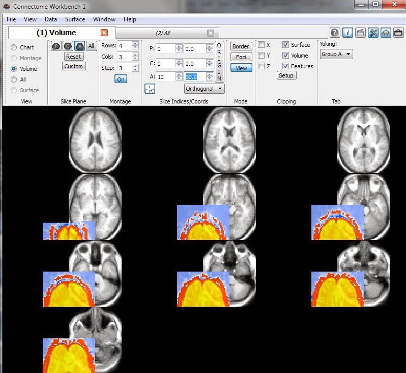
Here's another example of what a correctly-aligned file looks like: the NIfTI output image is displayed here as an overlay on a template anatomy in MRIcroN (overlay is red) and the Workbench (overlay is yellow). Note that the voxel value is correct (blue), and that the voxel's x,y,z coordinates (purple) match between the two programs. If you look closely, the voxel's i,j,k coordinates (blue) are 19,4,23 in MRIcroN (like they were in R), but 18,3,22 in the Workbench. This is ok: Workbench starts counting from 0, R and MRIcroN from 1.

concluding remarks

It's straightforward to combine the R code snippets above into loops that convert an entire dataset. My strategy is usually to step through the first image carefully - like in this post - then convert the images for the rest of the runs and participants in a loop (i.e., everyone with the same scanning parameters). I'll then open several other images, confirming they are aligned properly.

This last image is a concrete example of what you don't want to see: the functional data (colored overlay) is offset from the anatomical template (greyscale). Don't panic if you see this: dive back into the headers.

below-chance classification accuracy: meaningful here?

Below-chance accuracy ... always exciting. It showed up today in an interesting way in a set of control analyses. For framing, this is a bit of the working memory task data from the HCP: 0-back and 2-back task blocks, using pictures of faces or places as the stimuli. This gives four examples (volumetric parameter estimate images) per person: 0-back with faces, 0-back with places, 2-back with faces, and 2-back with places.

The classification shown here was with linear SVM, two classes (all balanced, so chance is 0.5), with leave-16-subjects-out cross-validation. The cross-validation is a bit unusual since we're aiming for generalizability across people: I trained the classifiers on a pair of stimuli in the training people, then tested on a different pair of stimuli in the testing people. For example, one cross-validation fold is training on 0-back vs 2-back face in 144 people, then testing 0-back vs 2-back place with the 16 left-out people.

Anyway, a ROI-based classification analysis was performed, on 6 anatomic clusters (C1:C6), which are along the x-axis in the graphs. The left side graph shows a positive control-type analysis: as we expected, face vs. place is classified extremely well with these ROIs, but 0-back vs. 2-back is classified at chance. The right side graph shows some non-sensical, negative control-type analyses, all of which we expected to classify around chance. These are nonsense because we're training and testing on different classifications: for example, training a classifier to distinguish face vs place, then testing with all face stimuli, some of which were from 0-back blocks, others of which were from 2-back blocks.

The striking pattern is that the blue and green lines are quite far below chance, particularly in clusters C1 and C2, which classified face vs place nearly perfectly (ie in the left-side graph).

These ROIs classify face vs place very well. When trained on face vs place, but tested with 0-back vs. 2-back (red and purple lines), they classified basically at chance. This makes sense, because the classifiers learned meaningful ways to distinguish face and place during training, but then were tested with all face or all place stimuli, which they presumably would have classified according to picture type, not n-back. This gives a confusion matrix like the one shown here: all face test examples properly classified as face, for 10/20 = 0.5 accuracy.

Now, the classifiers did not learn to classify 0-back vs 2-back in these ROIs (left-side graph above). To get the observed below-chance accuracies, the confusion matrices would need to be something like this. Why? It is sort of plausible that the classifier could "know" that the place test examples are not face, and so split them equally between the two classes. But if the classifier properly classifies all the 2-back face examples here (as needed to get the below-chance accuracy), why wasn't 0-back vs 2-back properly classified before?

I'll keep looking at this, and save some of the actual confusion matrices to see how exactly the below-chance accuracies are being generated. It's not quite clear to me yet, but the striking pattern in the below-chance here makes me think that they actually might carry some meaning in this case, and perhaps give some more general insights. Any thoughts?

some thoughts on "Generation and Evaluation of a Cortical Area Parcellation from Resting-State Correlations"

Lately I've been working a bit with the brain parcellation map described in Gordon, et al. (2014), "Generation and Evaluation of a Cortical Area Parcellation from Resting-State Correlations" (citation below), which is available from the authors (thanks!) in both surface and volumetric formats.

As the title of the paper states, their brain parcellation was derived from resting state functional connectivity analyses. Briefly, the paper describes defining a set of ROIs ("parcels") which divide the cortical surface into meaningful (structurally and functionally) units. The parcel boundaries were defined from functional connectivity analyses, following the (reasonable) assumption that functional connectivity statistics should be homogenous within a parcel, but shift abruptly at parcel boundaries.

This is not the first functional connectivity-derived brain parcellation (Table 1 of the paper lists others), but I think is probably the most methodologically rigorous to date. I like that they used two datasets, each with more than 100 people, and serious quality control checks (motion, etc). I also like their reliability/stability/validity analyses: both between the two datasets, in individuals, and against the most robust and best understood atlases (including cytoarchitechtonic).

We'd like to use the parcellation for defining ROIs, particularly for frontal and parietal areas that aren't definitively divided in existing atlases. Gordon et al. did their analyses on the surface, but provide both surface (CIFTI) and volumetric (NIfTI) versions of the parcellation.

Here's an image I made (using a version of my knitr plotting code) showing a few slices the volumetric parcels (plotted on a conte MNI anatomy I resampled to 2x2x2 mm voxels to match the parcellation's resolution). As is apparent, while in volumetric space, the parcels closely follow the cortical surface (grey matter ribbon).

I see the logic of constraining analyses to the surface, particularly when fMRI images are acquired with high-resolution imaging and then subjected to precise, surface-optimized preprocessing (such as in the HCP). But I'm less convinced these narrow ROIs are advantageous for datasets collected with larger voxels (say 3x3x3 mm or larger) and "standard" preprocessing (such as SPM and spatial normalization).

For example, here are a few slices showing some of the validated ROIs from my recent paper overlayed on a few greyscale slices from the Gordon et al. parcellation. My dataset was acquired with 4x4x4 mm voxels, and all preprocessing was volumetric. The red ROI in the image at left was defined using a volumetric searchlight analysis, and, unsurprisingly, is rather "blobby:" it's not constrained to the cortical ribbon. The red ROI contains 416 voxels, of which 181 (.43) are in one of the parcels. Does that mean the 235 non-parcel voxels are uninformative? No. With 4x4x4 mm voxels, typical amounts of movement, and preprocessing which included spatial normalization, some of the BOLD, even if it all actually came from the grey matter, will appear to come from outside the cortical ribbon.

To summarize, my take is that this parcellation is the result of a methodological tour de force and worth careful consideration, especially for a high-resolution dataset preprocessed with surface analysis in mind (e.g. with freesurfer), even if doing a volumetric analysis. It may be less suitable for datasets with larger voxels and more standard preprocessing.


Gordon EM, Laumann TO, Adeyemo B, Huckins JF, Kelley WM, & Petersen SE (2014). Generation and Evaluation of a Cortical Area Parcellation from Resting-State Correlations. Cerebral cortex. PMID: 25316338 doi:10.1093/cercor/bhu239