MVPA significance with the binomial test

Using the binomial test to evaluate significance is advocated by Francisco Pereira and Tom Mitchell (and others!); reference below. The method is easy to explain, but the exact implementation is not transparent to me: how to count the "number of correctly labeled test set examples" when I have multiple cross-validation folds, multiple subjects, and perhaps multiple repeats?

The common practice (as far as I can tell; I'll post your reply/comment if you disagree!) is to handle these problems by 1) counting the number of examples in the entire test set (summing over cross-validation folds) and 2) using the average over the multiple subjects and repeats as the number correct.

Here's an example in R:

# 3 runs, 10 examples in each (5 of two classes), 3 people
# here's how each person did:
(8 + 6 + 5)/30   # 19 correct, 0.6333333
(10 + 5 + 5)/30  # 20 correct, 0.6666667
(10 + 8 + 7)/30  # 25 correct, 0.8333333

# calculate the average accuracy for number correct
mean(c(0.6333333, 0.6666667, 0.8333333));   # 0.7111111
0.71 * 30  # 21.3 examples correct on average

# calculate the binomial test of the average. 
# have to round to a whole number correct.
binom.test(20, 30, 0.5) #  p-value = 0.09874

# calculating the binomial summing over the number of examples in
# all the subjects makes a much smaller p-value:
(8 + 6 + 5 + 10 + 5 + 5 + 10 + 8 + 7) # 64
binom.test(64, 90, 0.5);  # p-value = 7.657e-05

# t-test version (also common, though not directly comparable)
t.test(c(0.6333333, 0.6666667, 0.8333333), mu=0.5, alternative='greater'); # p-value = 0.03809

# binomial tests for each person.
binom.test(20, 30, 0.5)   # p-value = 0.09874
binom.test(19, 30, 0.5)   # p-value = 0.2005
binom.test(25, 30, 0.5)   # p-value = p-value = 0.0003249

While not the case in this toy example (if do the binomial on the average), I often find that the binomial produces smaller group p-values than the t-test or permutation testing. Nevertheless, I do not often use it, because so much information gets lost: variation between people, between test sets, between replications (if done).

It seems odd to use the across-subjects average and then have the exact same test (20 correct out of 30) regardless of whether there were 3 subjects or 300, but worse to sum over the number of examples in all the subjects (64 correct out of 90), because then the difference required for a significance is so small and the actual test set size is lost completely. It also 'feels' improper to me to use the total number of test set examples in all the cross-validation folds; even if all of the examples are fully independent the performance on the cross-validation folds certainly is not.

I am certainly not advocating that we ignore all research that used the binomial! But I do tend to interpret the significance levels that result with even more skepticism than usual.

Pereira, F., Mitchell, T., & Botvinick, M. (2009). Machine learning classifiers and fMRI: A tutorial overview NeuroImage, 45 (1) DOI: 10.1016/j.neuroimage.2008.11.007




see additional posts on this topic: 1

MVPA significance with the binomial test: update 1

A clarification is in order: in the previous post I imply that Francisco advocates using the binomial to test for significance across subjects as I illustrated in the R code. He doesn't. The code showing how to calculate the binomial for each person separately is the way he describes, though.

Francisco gives a few ideas in the "Group level analysis" section of his "Information Mapping" paper (citation below), mostly advocating descriptions or count-based techniques. This can work fairly well for searchlight analyses (e.g. map the proportion of subjects with each voxel significant), but not as well for ROI-based analyses like the toy example in the previous post. He'll be sharing some thoughts in a future post.


 Pereira F, & Botvinick M (2011). Information mapping with pattern classifiers: a comparative study. NeuroImage, 56 (2), 476-96 PMID: 20488249

research blogging: "Exceeding chance level by chance"

Neuroskeptic made me aware of a new paper by Combrisson & Jerbi entitled "Exceeding chance level by chance: The caveat of theoretical chance levels in brain signal classification and statistical assessment of decoding accuracy"; full citation below. Neuroskeptic's post has comments and a summary of the article, which I suggest you check out, along with its comment thread. 

My first reaction reading the article was confusion: are they suggesting we shouldn't test against chance (0.5 for two classes), but some other value? But no, they are arguing that it is necessary to do a test against chance ... to which I say, yes, of course it is necessary to do a statistical test to see if the accuracy you obtained is significantly above chance. The authors are arguing against a claim ("the accuracy is 0.6! 0.6 is higher than 0.5, so it's significant!") that I don't think I've seen in an MVPA paper, and would certainly question if I did. Those of us doing MVPA debate about how exactly to best do a permutation test (a favorite topic of mine!), and if the binomial or t-test is appropriate in particular situations, but everyone agrees that a statistical test is needed to support a claim that an accuracy is significant. In short, I agree with Nikolaus Kriegeskorte's comment that this is a strawman argument.

What about the results of the paper's analyses? Basically, they strike me as unsurprising. For example, the authors note that smaller datasets are less stable (eg quite easy to get accuracies above 0.7 in noise data when only 5 examples of each class), and that smaller test set sizes (eg leave-1-out vs. leave-20-out cross validation when 100 examples) tend to have higher variance across the cross-validation folds (and so harder to reach significance). At right is Figure 1e, showing the accuracies they obtained from classifying many (Gaussian random) noise datasets of different sizes. What I immediately noticed is how nice and symmetrical around chance the spread of dots appears: this is the sort of figure we expect to see when doing a permutation test. Eyeballing the graph (and assuming the permutation test was done properly), we'd probably end up with accuracies above 0.7 being significant at small sample sizes, and around 0.6 for larger datasets, which strikes me as reasonable.

I'm not a particular fan of using the binomial for significance in neuroimaging datasets, especially when the datasets have any sort of complex structure (eg multiple fMRI scanning runs, cross-validation, more than one person), which they almost always have. Unless your data is structured exactly like Combrisson & Jerbi's (and they did the permutation test properly, which they might not have, see Martin Hebart's comments), Table 1 strikes me as inadequate for establishing significance: I'd want to see a test taking into account the variance in your actual dataset (and claims being made).

Perhaps my concluding comment should be that proper statistical testing can be hard, and is usually time consuming, but is absolutely necessary. Neuroimaging datasets are nearly always structured (eg sources of variance and patterns of dependency and interaction) far differently from the assumptions of quick statistical tests, and we are asking questions of them not covered by one-line descriptions. Don't look for a quick fix, but rather focus on your dataset and claims, and a method for establishing significance levels is nearly always possible.

Combrisson, E., & Jerbi, K. (2015). Exceeding chance level by chance: The caveat of theoretical chance levels in brain signal classification and statistical assessment of decoding accuracy Journal of Neuroscience Methods DOI: 10.1016/j.jneumeth.2015.01.010

permuting searchlight maps: Stelzer

Now to the proposals in Stelzer, not just their searchlight shape!

This is a dense methodological paper, laying out a way (and rationale) to carry out permutation tests for group-level classifier-based searchlight analysis (linear svm). This is certainly a needed topic; as pointed out in the article, the assumptions behind t-tests are certainly violated in searchlight analysis, and using the binomial is also problematic (they suggest that it is too lenient, which strikes me as plausible).

Here's my interpretation of what they propose:

1. Generate 100 permuted searchlight maps for each person. You could think of all the possible label (i.e. class, stimulus type, whatever you're classifying) rearrangements as forming a very large pool. Pick 100 different rearrangements for each person and do the searchlight analysis with this rearrangement. (The permuted searchlight analysis must be done exactly as the real one was - same cross-validation scheme, etc.)
2. Generate 100,000 averaged group searchlight maps. Each group map is made by picking one permuted map from each person (out of the 100 made for each person in step 1) and averaging the values voxel-wise. In other words, stratified sampling with replacement.
3. Do a permutation test at each voxel, calculating the accuracy corresponding to a p = 0.001 threshold. In other words, at each voxel you record the 100th biggest accuracy after sorting the 100,000 accuracies generated in step 2. (100/100000 = 0.001)
4. Threshold the 100,000 permuted group maps and the one real-labeled group map using the voxel-wise thresholds calculated in step 3. Now the group maps are binary (pass the threshold or not).
5. Apply a clustering algorithm to all the group maps. They clustered voxels only if they shared a face. I don't think they used a minimum cluster size, but rather called un-connected voxels clusters of size 1 voxel. (This isn't really clear to me.)
6. Count the number of clusters by size in each of the 100,000 permuted maps and 1 real map. (this gives counts like 10 clusters with 30 voxels in map #2004, etc.)
7. Generate the significance of the real map's clusters using the counts made in step 6. I think they calculated the significance for each cluster size separately then did FDR, but it's not obvious to me ("Cluster-size statistics" section towards end of "Materials and Methods").
8. Done! The voxels passing step 7 are significant at the cluster level, corrected for multiple comparisons (Figure 3F of paper). The step 4 threshold map can be used for uncorrected p-values (Figure 3E of paper).

Most of this strikes me as quite reasonable. I've actually previously implemented almost this exact procedure (minus the cluster thresholding) on a searchlight dataset (not linear svms).

The part that makes me twitch the most is step 2: turning the 100 maps for each person into 100,000 group-average maps. I've been wanting to post about this anyway in the context of my ROI-based permutation testing example. But in brief, what makes me uncomfortable is the way 100 maps turn into 100000. Why not just calculate 5 for each person?  5^12 >> 100,000 (they had 12 subjects in some of the examples).  Somehow 100 for each person feels more properly random than 5 for each person, but how many are really needed to properly estimate the variation? I will expand on this more (and give a few alternatives), hopefully somewhat soon.

 The other thing that makes me wonder is the leniency. They show (e.g. Figure 11) that many more voxels are called significant in their method than with a t-test, claiming that as closer to the truth. This relates to my concern about how to combine over subjects: using 100,000 group maps allows very small p-values. But if the 100,000 aren't as variable as they should be, the p-values will be inflated.


Stelzer, J., Chen, Y., & Turner, R. (2012). Statistical inference and multiple testing correction in classification-based multi-voxel pattern analysis (MVPA): Random permutations and cluster size control. NeuroImage DOI: 10.1016/j.neuroimage.2012.09.063



UPDATE (30 October): We discussed this paper in a journal club and a coworker explained that the authors do explain the choice of 100 permutations per person in Figure 8 and the section "Undersampling of the permutation space". They made a dataset with one searchlight and many examples (80, 120, 160), then varied the number of permutations they calculated for each individual (10, 100, 1000, 10,000). They then made 100,000 group "maps" as before (my step 2), drawing from each group of single-subject permutations. Figure 8 shows the resulting histograms: the curves for 100, 1000, and 10,000 individual permutations are quite similar, which they use as rationale for running 100 permutations for each person (my step 1).

I agree that this is a reasonable way to choose a number of each-person permutations, but I'm still not entirely comfortable with the way different permutation maps are combined. I'll explain and show this more in a separate post.

searchlight shapes: Stelzer

This is the first of what will likely be a series of posts on a paper in press at NeuroImage:

Stelzer, J., et al., Statistical inference and multiple testing correction in classification-based multi-voxel pattern analysis (MVPA). NeuroImage (2012), http://dx.doi.org/10.1016/j.neuroimage.2012.09.063

There is a lot in this paper, touching some of my favorite topics (permutation testing, using the binomial, searchlight analysis, Malin's 'random' searchlights).
But in this post I'll just highlight the searchlight shapes used in the paper. They're given in this sentence: "The searchlight volumes to these diameters were 19 (D=3), 57 (D=5), 171 (D=7), 365 (D=9), and 691 (D=11) voxels, respectively." The authors don't list the software they used; I suspect it was custom matlab code.

Here I'll translate the first few sizes to match the convention I used in the other searchlight shape posts:

diameter	radius	number of surrounding voxels	notes
3	1	18	This looks like my 'edges or faces touch' searchlight.
5	2	56	This has more voxels than the 'default' searchlight, but less than my two-voxel radius searchlight. Squinting at Figure 1 in the text, I came up with the shape below.

Here's the searchlight from Figure 1, and my blown-up version for a two-voxel radius searchlight.

It looks like they added the plus signs to the outer edges of a three-by-three cube. This doesn't follow any of my iterative rules, but perhaps would result from fitting a particular sphere-type rule.

"Classification Based Hypothesis Testing in Neuroscience", permuting

My previous post described the below-chance classification part of a recent paper by Jamalabadi et. al; this post will get into the parts on statistical inference and permutation testing.

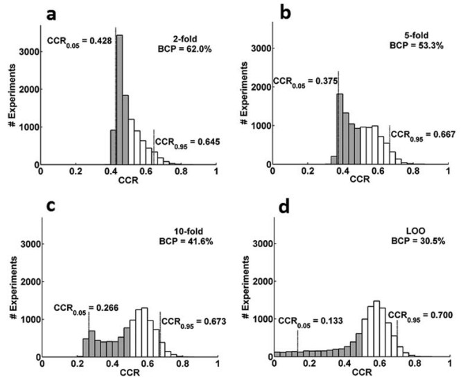
First, I fully agree with Jamalabadi et. al that MVPA classification accuracy (or CCR, "correct classification rate", as they call it) alone is not sufficient for estimating effect size or establishing significance. As they point out, higher accuracy is better, but it can only be directly compared within a dataset: the number of examples, classifier, cross-validation scheme, etc. all influence whether or not a particular accuracy is "good". Concretely, it is very shaky to interpret a study as "better" if it classified at 84% while a different dataset in a different study classified at 76%; if, however, you find that changing the scaling of a dataset improves classification (of a single dataset) from 76 to 84%, you'd be more justified in calling it an improvement.

The classification accuracy is not totally meaningless, but you need something to compare it to for statistical inference. As Jamalabadi et. al put it (and I've also long advocated), "We propose that MVPA results should be reported in terms of P values, which are estimated using randomization tests."{Aside: I think it's ok to use parametric tests for group-level inference in particular cases and after checking their assumptions, but prefer permutation tests and think they can provide stronger evidence.}

But there's one part of the paper I do not agree with, and that's their discussion of the prevalence of highly non-normal null distributions. The figure at left is Figure 5 from the paper, and are very skewed and non-normal null distributions resulting from classifying simulated datasets in different ways (chance should be 0.5). They show quite a few skewed null distributions from different datasets in the paper, and in the Discussion state that, "For classification with cross-validation in typical life-science data, i.e., small sample size data holding small effects, the distribution of classification rates is neither normal nor binomial."

However, I am accustomed to seeing approximately normal null distributions with MVPA, even in situations with very small effects and sample sizes. For example, below are null distributions (light blue) from eight simulated datasets. Each dataset was created to have 20 people, each with 4 runs of imaging data, each of which has 10 examples of each of 2 classes, and a single 50-voxel ROI. I generated the "voxel" values from a standard normal, with varying amounts of bias added to the examples of one class to allow classification. Classification was with leave-one-run-out cross-validation within each person, then averaging across the runs for the group-level accuracy; 1000 label rearrangements for the permutation test, following a dataset-wise scheme, averaging across subjects like in this demo.

The reddish line in each plot is the accuracy of the true-labeled dataset, which you can see increases from left to right across the simulated datasets, from 0.51 (barely above chance) to 0.83 (well above chance). The permutation test (perm. p) becomes more significant as the accuracy increases, since the true-labeled accuracy shifts to the right of the null distribution.

Note however, that the null distributions are nearly the same and approximately normal for all eight datasets. This is sensible: while the amount of signal in the simulated datasets increases, they all have the same number of examples, participants, classification algorithm (linear SVM, c=1), and cross-validation scheme. The different amounts of signal don't affect the permutation datasets: since the labels were randomized (within each subject and run), all permutation datasets are non-informative, and so produce similar null distributions. The null distributions above are for the group level (with the same dataset-wise permutation relabelings used within each person); I typically see more variability in individual null distributions, but with still approximate normality.

I suspect that the skewed null distributions obtained by Jamalabadi et. al are due either to the way in which the labels were permuted (particularly, that they might not have followed a dataset-wise scheme), or to the way the datasets were generated (which can have a big impact). Regardless, I have never seen as highly-skewed null distributions in real data as those reported by Jamalabadi et. al.



Jamalabadi H, Alizadeh S, Schönauer M, Leibold C, & Gais S (2016). Classification based hypothesis testing in neuroscience: Below-chance level classification rates and overlooked statistical properties of linear parametric classifiers. Human brain mapping, 37 (5), 1842-55 PMID: 27015748

Akama 2012: Decoding semantics across fMRI sessions

I want to highlight just a few methodology-type bits of Akama 2012 ("Decoding semantics across fMRI sessions with different stimulus modalities"); I encourage you to read the full paper for discussion of why they actually did the experiment (and what they made of it!).

accuracy over time

The main bit I want to highlight is Figure 4 ("Comparison between the model accuracy function and the canonical HRF in the range of 0–20 s after stimulus onset."):

Figure 4 shows the single-volume classification accuracy for each of the five participants (P1, P2, etc) and two stimulus modalities ("audio" and "ortho"), classifying whether the stimulus (in both modalities) was of a tool or an animal. They used a 1-second TR, and (I think) leave-one-run-out cross-validation, with six runs. They label the dashed horizontal line as "Chance Level" from a binomial test, which I think is rather lenient, but the accuracies are high enough that I won't quibble about significance (I'd just label 50% as chance, since it's two-class classification).

As the authors point out, the peak classification accuracy is closer to 7 seconds after onset in four of the participants, instead of 5, as in the default SPM HRF (thick red line). The lines are hard to see, but P5 (darkish purple) is the person with the most similarity between the canonical HRF and classification accuracy curves, for both modalities. The accuracy curves tend to be similar across modalities within participants, or, as they put it: "The main regularities were specific to participants, with correlations between the profiles of both conditions of 0.88 for P1, 0.72 for P2, 0.81 for P3, 0.91 for P4, and 0.96 for P5."

This is the nicest figure I've seen showing how accuracy increases over time and varies over people; the scanning parameters and experimental design let the authors calculate this at a higher resolution than usual. This figure will be going into my introduction-to-MVPA slides.

cross-modal comments

The experiment had two sessions (I think on separate days, though this isn't clear): one in which images of hand tools and animals (same each modality) were accompanied by auditory labels ("audio") and the other, with written labels ("ortho"). Classification was of image category (tool or animal), and was done either with a single session's data (all audio or all ortho), or cross-session (cross-modal), training with audio and testing with ortho, or training with ortho and testing with audio. Classification accuracies were pretty high both times (figures 2 and 3), but higher within- than cross-modality, and the authors spend some time exploring and  discussing possible reasons why. Here are a few more ideas.

A new experiment could be run, in which both audio and ortho stimuli are presented in each session (e.g. three runs of each on each day). Is cross-modal classification less accurate than within-modal, or is cross-session accuracy less than within-session accuracy? In other words, I expect analyses involving images collected on separate days to be less accurate than analyses with images collected within a single session, simply because time has passed (the scanner properties could change a bit, the person could have different hydration or movement, etc). It's not possible to sort out the session and modality effects in Akama 2012, since they're confounded.

Also, I wonder if the feature selection method (picking top 500 voxels by ANOVA ranking in training set) hurt the likelihood of finding strong cross-modal classification. A ROI-based analysis might be an appropriate alternative, particularly since Tool vs. Animal classification has been studied before.



Hiroyuki Akama, Brian Murphy, Li Na, Yumiko Shimizu, & Massimo Poesio (2012). Decoding semantics across fMRI sessions with different stimulus modalities: a practical MVPA study Frontiers in NeuroInformatics DOI: 10.3389/fninf.2012.00024

permutation schemes: leave-one-subject-out

I've posted before about permutation schemes for the group level; here's an explicit illustration of the case of leave-one-subject-out cross-validation, using a version of these conventions. I'm using "leave-one-subject-out" as shorthand to refer to cross-validation in which partitioning is done on the participants, as illustrated here.

This diagram illustrates a fMRI dataset from two tasks and four participants, with one example of each task per person. Since there are four participants there are four cross-validation folds; here, the arrows indicate that for the first fold the classifier is trained on data from subjects 2, 3, and 4, while subject 1's data makes up the test set. The overall mean accuracy results from averaging the four accuracies (see this for more explanation).

How to get a significance value for the overall mean accuracy (grey oval)? We can't just do a t-test (or binomial) over the accuracies we got by leaving out each person (as often done after within-subjects classification), because the accuracies are not at all independent: we need a test for the final mean accuracy itself.

My strategy is to do dataset-wise permutation testing by label-flipping within one or more participants each fold. In this case, there are only four participants, so we could flip labels in just one or two of the participants, for 10 possible permutations (choose(4,1) + choose(4,2)) (flipping all the subjects' labels would recreate the original dataset, since this is dataset-wise permutation testing.) Here, the task labels for participant 1 only are flipped (the first example becomes task 2, the second, task 1). The entire cross-validation then proceeds with each flipped-labels dataset.

 I follow the same strategy when there are more than one example of each class per person: when the person's labels are to be 'flipped' for a permutation I relabel all the class 1 examples as class 2 (and class 2 as class 1). While the number of possible permutations is limited by number of participants in this scheme, it increases rapidly with the number of participants.

Anyone do anything different?

a nice "Primer on Pattern-Based Approaches to fMRI"

John-Dylan Haynes has a new MVPA review article out in Neuron, "A Primer on Pattern-Based Approaches to fMRI" (full citation below). I say "new" because he (and Rees) was the author of one of the first MVPA overview articles ("Decoding mental states from brain activity in humans"), back in 2006. As with the earlier article, this is a good introduction to some of the main methods and issues; I'll highlight a few things here, in no particular order.

At left is part of Figure 4, which nicely illustrates four different "temporal selection" options for event-related designs. The red and green indicate the two different classes of stimuli (cats and dogs), with the black line the fMRI signal in a single voxel across time.

I often refer to these as "temporal compression" options, but like "temporal selection" even better: we are "selecting" how to represent the temporal aspect of the data, and "compression" isn't necessarily involved.

John-Dylan Haynes (quite properly, in my opinion) recommends permutation tests (over binomial and t-tests) for estimating significance, noting that one of their (many) benefits is in detecting biases or errors in the analysis procedure.

Overall, I agree with his discussion of spatial selection methods (Figure 3 is a nice summary), and was intrigued by the mention of wavelet pyramids as a form of spatial filtering. I like the idea of spatial filtering to quantify the spatial scale at which information is present, but haven't run across a straightforward implementation (other than searchlight analysis); wavelet pyramids might need more investigation.

I also appreciate his caution against trying too many different classifiers and analysis procedures on the same dataset, pointing out that this can cause "circularity and overfitting". This problem is also sometimes referred to as having too many experimenter degrees of freedom: if you try enough versions of an analysis you can probably find one that's "significant." His advice to use nested cross-validation strategies (e.g., tuning the analysis parameters on a subset of the subjects) is solid, if sometimes difficult in practice because of the limited number of available subjects. The advice to use an analysis that "substantially decreases the number of free parameters" is also solid, if somewhat unsatisfying: I often advise people to use linear SVM, c=1 as the default analysis. While tuning parameters and testing other classifiers could conceivably lead to a higher accuracy, the risk of false positives from exploiting experimenter degrees of freedom is very real.

I also like his inclusion of RSA and encoding methods in this "primer". Too often we think of classifier-based MVPA, RSA, and encoding methods as unrelated techniques, but it's probably more accurate to think of them as "cousins," or falling along a continuum.

It's clear by now that I generally agree with his issue framing and discussion, though I do have a few minor quibbles, such as his description of MVPA methods as aimed at directly studying "the link between mental representations and corresponding multivoxel fMRI activity patterns". I'd assert that MVPA are also useful as a proxy for regional information content, even without explicit investigation of cognitive encoding patterns. But these are minor differences; I encourage you to take a look at this solid review article.


  Haynes JD (2015). A Primer on Pattern-Based Approaches to fMRI: Principles, Pitfalls, and Perspectives. Neuron, 87 (2), 257-70 PMID: 26182413