demo: R code to perform a voxelwise t-test

It's easy to perform a voxelwise t-test (t-test at each voxel individually). Programs for mass-univariate analysis (like SPM and fsl) of course do this (and much more), but sometimes you just want to do a simple t-test across subjects at each voxel.

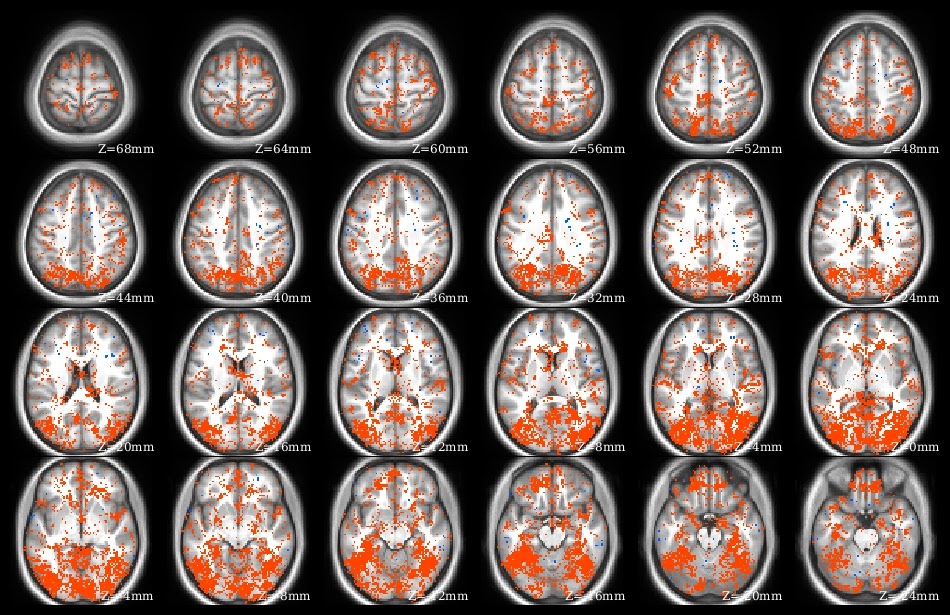
The demo code linked in this post does a voxelwise t-test in R. It takes as input a set of 3d NIfTI files, where each NIfTI is assumed to come from a different person, each voxel of which contains a statistic describing effect strength (for example, accuracy resulting from a searchlight analysis). The code reads the 3d NIfTI images into a 4d array (people in the fourth dimension), then performs a t-test at each voxel, saving the t-values for each voxel in a new NIfTI image. This figure shows the t-value image produced by the demo code.

UPDATE 4 June 2021:

The original version of this post continues below. I wrote a new version of the code to 1) avoid aaply (memory usage a bit better), and 2) use the RNifti instead of oro.nifti library (RNifti functions can be dramatically faster, and have some nice features; I now use RNifti exclusively for nifti image R input/output). I also added the files to the MVPA Meanderings OSF site, under the "voxelwise" subdirectory (direct link to R script).

Both versions of this code loop through all of the image voxels, which is most assuredly not the most efficient (or foolproof) way to perform a voxelwise t-test (I would recommend 3dttest++ instead, perhaps following 3dbucket; calling afni functions directly from R can make things quite smooth for those of us that are not bash fluent). I rewrote rather than removed this demo, however, because sometimes looping through all the voxels like this is the most straightforward way to get something done. 

Connectome Workbench: 1st Steps

Here's my advice for getting started with the Connectome Workbench:

1. First, go through my tutorial on getting started with Workbench: it describes downloading Workbench, starting it, loading images, and viewing overlay and underlay images.
2. This tutorial introduces wb_command, and shows how to use it to create a surface file from a volumetric NIfTI (for quick-viewing purposes, not for further analysis).
3. Read my summary of the different file types.
4. Try the official Workbench tutorial (or at least look through the manual to get an idea of the possibilities).
5. Look at my post on using the Workbench with volumetric images.

And why bother learning Workbench? Setting aside all its surface and CCF/HCP functionality (and that's a lot to set aside), I think the ability to create "scenes" justifies the time spent learning the software.

This screenshot shows scenes in action: clicking the little button marked with yellow arrows brings up the scene dialog box. I have three scenes stored in this file, and selecting one for display changes Workbench to recreate exactly how it was when the scene was created: window size, colors and scaling, loaded images, tab layout. Creating scenes for each image that might be used in a publication can save massive amounts of time: need to adjust a threshold or change a color? Just bring up the scene and make the change, no need to start from the beginning.



 UPDATE 26 March 2020: linked to the new getting-started tutorial.
UPDATE 8 February 2018: linked to the new volume to surface tutorial; fixed the official tutorial link.
UPDATE 2 August 2017: removed the (very outdated!) mention of the release of Connectome Workbench 1.0; renamed this post to the more general "Connectome Workbench: 1st Steps".

nice methods: Manelis and Reder 2013, "He Who is Well Prepared ..."

It's always great to read a paper with interesting methodology clearly explained, and Manelis and Reder 2013, "He Who Is Well Prepared Has Half Won The Battle: An fMRI Study of Task Preparation" is one of those papers (full citation below). As usual, I'm not going to fully describe the paper (go read it!), but just comment on a few things that caught my eye.




First, I was struck again by the strength and consistency of the activations and deactivations associated with the n-back task; they seem as reliable as those from some motor and somatosensory tasks. The authors used a mass-univariate analysis to identify a set of ROIs to use for the MVPA, shown in this part of Figure 2 (warm colors for regions that increased with n-back level, and cool colors for regions that decreased). As the authors properly point out, doing MVPA on the task blocks with these ROIs would be somewhat circular (since a mass-univariate analysis of the task blocks was used to create the ROIs), but their main MVPA avoids circularity, since it was done on a different part of the task.

Next, I appreciated the discussions of possible confounds in the results section: the authors report pairwise accuracies, not just the three-way, explaining that they want to make sure one very accurate pair is not driving the results, and they performed a nice control analysis using randomly-selected rest volumes.

Finally, they found a correlation between classification accuracy (MVPA during task preparation periods) and behavioral performance (participant speed on the n-back task); there are still relatively few reports tying fMRI analyses to behavior, and it's nice to see another one.


Manelis, A., & Reder, L. (2013). He Who Is Well Prepared Has Half Won The Battle: An fMRI Study of Task Preparation Cerebral Cortex DOI: 10.1093/cercor/bht262

quick recommendation: pre-calculate permutation test schemes

A quick recommendation: I strongly suggest pre-calculating the relabeling schemes before running a permutation test. In other words, prior to actually running the code doing all the calculations necessary to generate the null distribution, determine which relabeling will be used for each iteration of the permutation test, and store these new labels so that they can be read out again. To be clear, I think the only alternative to pre-calculating the relabeling scheme is to generate them at run time, such as by randomly resampling a set of labels during each iteration of the permutation test; that's not what I'm recommending here.

There are several reasons I think this is a good principle to follow for any "serious" permutation test (e.g. one that might end up in a publication):

Safety and reproducibility. It's a lot easier to confirm that the relabeling scheme is operating as expected when it can be checked outside of debug mode/run time. At minimum, I check that there are no duplicate entries, and that the randomization looks reasonable (e.g. labels chose at approximately equal frequencies?). Having the relabeling stored also means that the same permutation test can be run at a later time, even if the software or machines have changed (built-in randomization functions are not always guaranteed to produce the same output with different machines or versions of the software).

Easy of separating the jobs. I am fortunate to have access to an excellent supercomputing cluster. Since my permutations are pre-calculated, I can run a permutation test quickly by sending many separate, non-interacting jobs to the different cluster computers. For example, I might start one job that runs permutations 1 to 20, another job running permutations 21 to 30, etc. In the past I've tried running jobs like this by setting random seeds, but it was much more buggy than explicitly pre-calculating the labelings. Relatedly, if a job crashes for some reason it's a lot better to be able to start after the last-completed permutation if they've been pre-calculated.

more on the LD-t

In a previous post I wrote a bit about  A Toolbox for Representational Similarity Analysis, and my efforts at figuring out the LD-t statistic. Nikolaus Kriegeskorte kindly pointed me to some additional information, and cleared up some of my confusion. Note that I'll be using the term "LD-t" in this post for consistency (and since it's short); it's a "cross-validated, normalized variation on the Mahalanobis distance", as phrased in Nili (2014).

First, the LD-t has been described and used previously (before Nili et al 2014), though (as far as I can tell) not in the context of representational similarity analysis (RSA). It is summarized in this figure (Figure S8a from Kriegeskorte et al. (2007 PNAS)); the paper's supplemental text has additional explanation ("Significance testing of ROI response-pattern differences" section). A bit more background is also on pages 69-71 of Niko's thesis.

To give a high-level picture, calculating the LD-t involves deriving a t-value from Fisher linear discriminant test set output. The linear discriminant is fit (weights calculated from the training data) with the standard algorithms, but using an error covariance matrix calculated from the residuals of fitting a GLM to the entire training dataset (time-by-voxel data matrix), which is then run through the Ledoit-Wolf Covariance Shrinkage Estimator function.

This isn't a procedure that can be dropped into an arbitrary MVPA workflow. For example, for my little classification demo I provided a single-subject 4D dataset, in which each of the 20 volumes is the temporally-compressed version (averaging, in this case) of an experimental block; the first ten class A, the second ten class B. The demo then uses cross-validation and an SVM to get an accuracy for distinguishing class A and B. It is trivial to replace SVM in that demo with LDA, but that will not produce the LD-t. One reason is that the LD-t procedure requires splitting the dataset into two parts (a single training and testing set), not arbitrary cross-validation schemes, but there are additional differences.

Here's a description of the procedure; many thanks to Carolina Ramirez for guiding me through the MATLAB! We're assuming a task-based fMRI dataset for a single person.

• Perform "standard" fMRI preprocessing: motion correction, perhaps also slice-timing correction or spatial normalization. The values resulting from this could be output as a 4d data matrix of the same length as the raw data: one (preprocessed) image for each collected TR. We can also think of this as a (very large) time-by-voxel data matrix, where time is the TR.
• Create design matrices (X) for each half of the dataset (A and B, using the terms from the Toolbox file fisherDiscrTRDM.m). These are as usual for fMRI mass-univariate analysis: the columns generally includes predictors for motion and linear trends as well as the experimental conditions, which have been convolved with a hemodynamic response function.
• Create data matrices (Y) for each half of the dataset (training (A) and testing (B)), structured as usual for fMRI mass-univariate analysis, except including just the voxels making up the current ROI.
• Now, we can do the LD-t calculations; this is function fishAtestB_optShrinkageCov_C, also from the Toolbox file fisherDiscrTRDM.m. First, fit the linear model to dataset A (training data): 

eBa=inv(Xa'*Xa)*Xa'*Ya; % calculate betas
eEa=Ya-Xa*eBa; % calculate error (residuals) matrix

• Use the training set residuals matrix (eEa) to estimate the error covariance, and apply the Ledoit-Wolf Covariance Shrinkage Estimator function to the covariance matrix.This is Toolbox file covdiag.m, and returns the the shrinkage estimate of the covariance matrix, Sa.
• Use the inverse of that covariance matrix (invSa) and the training-set PEIs (eBa) to calculate the Fisher linear discriminant (C is a contrast matrix, made up of -1, 0, and 1 entries, corresponding to the design matrix). Fitting the discriminant function produces a set of weights, one for each voxel.

was=C'*eBa*invSa; % calculate linear discriminant weights

• Now, project the test dataset (Yb) onto this discriminant: yb_was=Yb*was'; 
• The final step is to calculate a t-value describing how well the discriminant separated the test set. t-values are a number divided by its standard error, which is the purpose of the final lines of the fishAtestB_optShrinkageCov_C function. The values are adjusted before the t-value calculation; it looks like this is intended to compensate for differing array dimensions (degrees of freedom). I don't fully understand each line of code, but here they are, for completeness:

invXTXb=inv(Xb'*Xb);
ebb_was=invXTXb*(Xb'*yb_was); 
eeb_was=yb_was-Xb*ebb_was;  
nDFb=size(yb_was,1)-size(Xb,2);
esb_was=diag(eeb_was'*eeb_was)/nDFb;
C_new=C(1:min([size(ebb_was,1),size(C,1)]),:);
ctb_was2=diag(C_new'*ebb_was);
se_ctb_was2=sqrt(esb_was.*diag(C_new'*invXTXb*C_new));
ts=ctb_was2./se_ctb_was2;

• Once the t-value is calculated it can be converted to a p-value if desired, using the standard t-distribution.

This procedure is for a single subject. For group analysis, in Kriegeskorte et al. (2007) they did a group analysis by "concatenating the discriminant time courses of all subjects and fitting a composite design matrix with separate predictors for each subject." Nili et al. (2014, supplemental) suggests a different approach: averaging the LD-t RDMs cell-wise across people, then dividing by the square root of the number of subjects.

The statistic produced by these calculations is related to the cross-validated MANOVA described by Carsten Allefeld; I hope to compare them thoroughly in the future.

King 2014: MEG MVPA and temporal generalization matrices

Last week at ICON I attended an interesting talk by Stanislas Dehaene, in which he described some work in recent papers by Jean-Rémi King; I'll highlight a few aspects (and muse a bit) here.

First, MVPA of MEG data. I've never worked with MEG data, but this paper (citation below) describes classifying (linear SVM, c=1!) trial type within-subjects, using amplitude in each of the 306 MEG sensors instead of BOLD in voxels (using all the MEG sensors is a whole-brain analysis: features span the entire brain). I should go back to (as the authors do here) referring to "MVPA" as an acronym for "multivariate pattern analysis" instead of "multi-voxel pattern analysis" to not exclude MEG analyses!

Second, I was quite taken with what they call "temporal generalization matrices", illustrated in their Figure 1, shown at left. These matrices succinctly summarize the results of what I'd call "cross-timepoint classification": rather than doing some sort of temporal compression to get one summary example per trial, they classify each timepoint separately (e.g. all the images at onset - 0.1 seconds; all the images at onset + 0.1 seconds). Usually I've seen this sort of analysis plotted as  accuracy at each timepoint, like Figure 3 in Bode & Haynes 2009.

"Temporal generalization matrices" take timepoint-by-timepoint analyses a step further: instead of training and testing on images from the same timepoint, they train on images from one timepoint, then test on images from every other timepoint, systematically. The axes are thus (within-trial) timepoint, training-set timepoint on the y-axis and testing-set timepoint on the x-axis. The diagonal is from training and testing on the same timepoint, same as the Bode & Haynes 2009-style line graphs.

Since this is MEG data, there are a LOT of timepoints, giving pretty matrices like these, taken from Figure 3. In the left-side matrix the signal starts around 0.1 seconds (bottom left corner of the red blotch) and lasts until around 0.4 seconds, without much generalization - a classifier trained at timepoint 0.2 won't accurately classify timepoint 0.4. The right-side matrix has much more generalization: a classifier trained at timepoint 0.2 classified all the way to the end of the trial. Altogether, these matrices are nice summaries of a huge number of classifications.

Finally, note the dark blue blotch in the left-side matrix: they found clear below-chance accuracy for certain combinations of timepoints, which they discuss quite a bit in the manuscript. I'm pointing this out since below-chance accuracies are a persistent issue, and they (properly) didn't over-interpret (or hide) it in this case.


King JR, Gramfort A, Schurger A, Naccache L, & Dehaene S (2014). Two distinct dynamic modes subtend the detection of unexpected sounds. PLoS One, 9 (1) PMID: 24475052

A toolbox for representational similarity analysis (and some RSA musings)

An interesting new paper about RSA, A Toolbox for Representational Similarity Analysis (Nili et al 2014, see citation below), shifted my picture of RSA a bit, making me realize I haven't always used the technique quite properly.

First, as you'd guess from the title, the paper mostly describes a MATLAB package for performing RSA. I could easily download the package and start looking at the demos and documentation, but there is a lot in the package, and understanding what all it's capable of (and how exactly it's doing everything) is not a job for an hour or two. It certainly looks worth careful examination, though; I'm particularly interested in the statistical inference functions.

The part I mostly want to comment on is separate from the MATLAB package: the paper suggests using a linear discriminant analysis t-value as a distance (dissimilarity) metric measure of discriminability instead of Pearson correlation (1 - Pearson correlation was suggested in Kriegeskorte 2008). Here's how they describe the method (there's a bit more in the supplemental):

"We first divide the data into two independent sets. For each pair of stimuli, we then fit a Fisher linear discriminant to one set, project the other set onto that discriminant dimension, and compute the t value reflecting the discriminability between the two stimuli. We call this multivariate separation measure the linear-discriminant t (LD-t) value."

This is dense. To unpack it a bit, the idea is that you're using a statistic derived from a classification analysis for the distance metric. They suggest using Fisher linear discriminant analysis (LDA) for the classification algorithm, with two-fold cross-validation, averaging results across the folds. LDA strikes me as a reasonable suggestion, and I assume any sort of reasonable cross-validation scheme (e.g. leave-one-run-out) would be fine.

But, how to derive the a t-value from the cross-validated LDA? The paper's description wasn't detailed enough for me, so I poked around in the toolbox code, and found the fishAtestB_optShrinkageCov_C function in /Engines/fisherDiscrTRDM.m. It looks like they're fitting the discriminant to the training dataset, projecting the test dataset onto the discriminant, then doing a t-test on the "error variance" computing a t-value from the test data projected on the discriminant. The function code does everything with linear algebra; my MATLAB (and linear algebra) is too rusty for it to all be obvious (e.g. which step, if any, corresponds to the coefficients produced by the R lda command? Is it a two-sided t-test against zero?). Please comment or email if you can clarify and I'll update this post. See this new post.

Anyway, the idea of using a classification-derived distance metric for RSA is appealing, particularly to get a consistent and predictable zero when stimuli are truly unrelated (fMRI examples are often a bit correlated, making correlation-based RSA comparisons sometimes between "not that correlated" and "somewhat correlated", rather than the more interpretable "nothing" and "something").

Which brings me to what I realized I had wrong about RSA. To do cross-validation, you need multiple examples of the same stimulus, and at the end you have a single number (accuracy, LD-t, whatever). RSA is accordingly not done between examples (e.g. individual trials) but between stimulus types (classes with lots of examples; what we classify).

This RSA matrix (the official term is "RDM") is from a previous post, which I described as "an RSA matrix for a dataset with six examples in each of two classes (w and f)." While the matrix is sensible (w-f cells are oranger - less correlated - than w-w and f-f cells), the matrix should properly be a single value: the distance between w and f.

In other words, to make an RSA matrix (RDM) I needed at least three classes; not multiple examples of two classes. Say the new class is 'n'. Then, my RSA matrix would have w, f, and n along each axis, and we can ask questions like, "is w is more similar to f or n?". That RSA matrix would have just three numbers: the distances between w and f, w and n, and f and n. If using Pearson correlation, we'd calculate those three numbers by averaging (or some other sort of temporal compression, such as fitting a linear model) across the examples of each class (here, w1, w2, w3, w4, w5, w6) to get one example per class, then correlating these vectors (e.g. w with f). If using LDA, we'd (for example) use the first three w and f examples to train the classifier, then test on the last three of each (and the reverse), then calculate the LD-t. (To be clear, you can calculate LD-t with just two classes, it won't really look like an RDM since you just have one value (w-f).)


Nili H, Wingfield C, Walther A, Su L, Marslen-Wilson W, & Kriegeskorte N (2014). A toolbox for representational similarity analysis. PLoS computational biology, 10 (4) PMID: 24743308

UPDATE 17 July 2014: Changed a bit of the text (strikeouts) in response to helpful comments from Hamed Nili. He also pointed out this page, which describes a few other aspects of the paper and toolbox.

UPDATE 21 August 2014: see this post for a detailed description of how to calculate the LD-t.